CFA 2019 Level 1 SchweserNotes Book 2

(1)

(2)

STUDY SESSION 4

The topical coverage corresponds with the following CFA Institute assigned reading:

14. Topics in Demand and Supply Analysis

The candidate should be able to:

a. calculate and interpret price, income, and cross-price elasticities of demand and describe factors that affect each measure. (page 1)

b. compare substitution and income effects. (page 7)

c. distinguish between normal goods and inferior goods. (page 7) d. describe the phenomenon of diminishing marginal returns. (page 8)

e. determine and interpret breakeven and shutdown points of production. (page 10) f. describe how economies of scale and diseconomies of scale affect costs. (page 13) The topical coverage corresponds with the following CFA Institute assigned reading:

15. The Firm and Market Structures

a. describe characteristics of perfect competition, monopolistic competition, oligopoly, and pure monopoly. (page 19)

b. explain relationships between price, marginal revenue, marginal cost, economic profit, and the elasticity of demand under each market structure. (page 22) c. describe a firm’s supply function under each market structure. (page 42)

d. describe and determine the optimal price and output for firms under each market structure. (page 22)

e. explain factors affecting long-run equilibrium under each market structure. (page 22)

f. describe pricing strategy under each market structure. (page 42)

g. describe the use and limitations of concentration measures in identifying market structure. (page 43)

h. identify the type of market structure within which a firm operates. (page 44) The topical coverage corresponds with the following CFA Institute assigned reading:

16. Aggregate Output, Prices, and Economic Growth

a. calculate and explain gross domestic product (GDP) using expenditure and income approaches. (page 51)

b. compare the sum-of-value-added and value-of-final-output methods of calculating GDP. (page 52)

c. compare nominal and real GDP and calculate and interpret the GDP deflator. (page 53)

d. compare GDP, national income, personal income, and personal disposable income. (page 54)

e. explain the fundamental relationship among saving, investment, the fiscal balance, and the trade balance. (page 56)

f. explain the IS and LM curves and how they combine to generate the aggregate demand curve. (page 58)

(11)

h. explain causes of movements along and shifts in aggregate demand and supply curves. (page 63)

i. describe how fluctuations in aggregate demand and aggregate supply cause short-run changes in the economy and the business cycle. (page 67)

j. distinguish between the following types of macroeconomic equilibria: long-run full employment, short-run recessionary gap, short-run inflationary gap, and short-run stagflation. (page 67)

k. explain how a short-run macroeconomic equilibrium may occur at a level above or below full employment. (page 67)

l. analyze the effect of combined changes in aggregate supply and demand on the economy. (page 70)

m. describe sources, measurement, and sustainability of economic growth. (page 72) n. describe the production function approach to analyzing the sources of economic

growth. (page 73)

o. distinguish between input growth and growth of total factor productivity as components of economic growth. (page 74)

17. Understanding Business Cycles

a. describe the business cycle and its phases. (page 83)

b. describe how resource use, housing sector activity, and external trade sector activity vary as an economy moves through the business cycle. (page 84) c. describe theories of the business cycle. (page 87)

d. describe types of unemployment and compare measures of unemployment. (page 89)

e. explain inflation, hyperinflation, disinflation, and deflation. (page 90) f. explain the construction of indexes used to measure inflation. (page 91) g. compare inflation measures, including their uses and limitations. (page 93) h. distinguish between cost-push and demand-pull inflation. (page 95)

(12)

STUDY SESSION 5

18. Monetary and Fiscal Policy

a. compare monetary and fiscal policy. (page 105)

b. describe functions and definitions of money. (page 106) c. explain the money creation process. (page 107)

d. describe theories of the demand for and supply of money. (page 108) e. describe the Fisher effect. (page 110)

f. describe roles and objectives of central banks. (page 110)

g. contrast the costs of expected and unexpected inflation. (page 112) h. describe tools used to implement monetary policy. (page 114) i. describe the monetary transmission mechanism. (page 114) j. describe qualities of effective central banks. (page 115)

k. explain the relationships between monetary policy and economic growth, inflation, interest, and exchange rates. (page 116)

l. contrast the use of inflation, interest rate, and exchange rate targeting by central banks. (page 117)

m. determine whether a monetary policy is expansionary or contractionary. (page 118)

n. describe limitations of monetary policy. (page 119) o. describe roles and objectives of fiscal policy. (page 121)

p. describe tools of fiscal policy, including their advantages and disadvantages. (page 122)

q. describe the arguments about whether the size of a national debt relative to GDP matters. (page 125)

r. explain the implementation of fiscal policy and difficulties of implementation. (page 126)

s. determine whether a fiscal policy is expansionary or contractionary. (page 127) t. explain the interaction of monetary and fiscal policy. (page 128)

19. International Trade and Capital Flows

a. compare gross domestic product and gross national product. (page 138) b. describe benefits and costs of international trade. (page 138)

c. distinguish between comparative advantage and absolute advantage. (page 139) d. compare the Ricardian and Heckscher–Ohlin models of trade and the source(s) of

comparative advantage in each model. (page 141)

e. compare types of trade and capital restrictions and their economic implications. (page 142)

(13)

g. describe common objectives of capital restrictions imposed by governments. (page 147)

h. describe the balance of payments accounts including their components. (page 148) i. explain how decisions by consumers, firms, and governments affect the balance of

payments. (page 149)

j. describe functions and objectives of the international organizations that facilitate trade, including the World Bank, the International Monetary Fund, and the World Trade Organization. (page 150)

20. Currency Exchange Rates

a. define an exchange rate and distinguish between nominal and real exchange rates and spot and forward exchange rates. (page 159)

b. describe functions of and participants in the foreign exchange market. (page 161) c. calculate and interpret the percentage change in a currency relative to another

currency. (page 162)

d. calculate and interpret currency cross-rates. (page 163)

e. convert forward quotations expressed on a points basis or in percentage terms into an outright forward quotation. (page 164)

f. explain the arbitrage relationship between spot rates, forward rates, and interest rates. (page 165)

g. calculate and interpret a forward discount or premium. (page 165)

h. calculate and interpret the forward rate consistent with the spot rate and the interest rate in each currency. (page 166)

i. describe exchange rate regimes. (page 168)

(14)

Video covering this content is available online. The following is a review of the Economics (1) principles designed to address the learning outcome statements set forth by CFA Institute. Cross-Reference to CFA Institute Assigned Reading #14.

READING 14: TOPICS IN DEMAND AND

SUPPLY ANALYSIS

Study Session 4

EXAM FOCUS

The Level I Economics curriculum assumes candidates are familiar with concepts such as supply and demand, utility-maximizing consumers, and the product and cost curves of firms. CFA Institute has posted three assigned readings to its website as prerequisites for Level I Economics. If you have not studied economics before (or if it has been a while), you should review these readings, along with the video instruction, study notes, and review questions for each of them in your online Schweser Candidate Resource Library to get up to speed.

MODULE 14.1: ELASTICITY

LOS 14.a: Calculate and interpret price, income, and cross-price elasticities of demand and describe factors that affect each measure.

CFA® Program Curriculum, Volume 2, page 9

Own-Price Elasticity of Demand

Own-price elasticity is a measure of the responsiveness of the quantity demanded to a change in price. It is calculated as the ratio of the percentage change in quantity

demanded to a percentage change in price. With downward-sloping demand (i.e., an increase in price decreases quantity demanded), own-price elasticity is negative. When the quantity demanded is very responsive to a change in price (absolute value of elasticity > 1), we say demand is elastic; when the quantity demanded is not very responsive to a change in price (absolute value of elasticity < 1), we say that demand is inelastic. In Figure 14.1, we illustrate the most extreme cases: perfectly elastic demand (at any higher price, quantity demanded decreases to zero) and perfectly inelastic demand (a change in price has no effect on quantity demanded).

(15)

When there are few or no good substitutes for a good, demand tends to be relatively inelastic. Consider a drug that keeps you alive by regulating your heart. If two pills per day keep you alive, you are unlikely to decrease your purchases if the price goes up and also quite unlikely to increase your purchases if price goes down.

When one or more goods are very good substitutes for the good in question, demand will tend to be very elastic. Consider two gas stations along your regular commute that offer gasoline of equal quality. A decrease in the posted price at one station may cause you to purchase all your gasoline there, while a price increase may lead you to purchase all your gasoline at the other station. Remember, we calculate demand and elasticity while holding the prices of related goods (in this case, the price of gas at the other station) constant.

Other factors affect demand elasticity in addition to the quality and availability of substitutes:

Portion of income spent on a good. The larger the proportion of income spent on a good, the more elastic an individual’s demand for that good. If the price of a preferred brand of toothpaste increases, a consumer may not change brands or adjust the amount used if the customer prefers to simply pay the extra cost. When housing costs increase, however, a consumer will be much more likely to adjust consumption, because rent is a fairly large proportion of income.

Time. Elasticity of demand tends to be greater the longer the time period since the price change. For example, when energy prices initially rise, some adjustments to consumption are likely made quickly. Consumers can lower the thermostat

temperature. Over time, adjustments such as smaller living quarters, better

insulation, more efficient windows, and installation of alternative heat sources are more easily made, and the effect of the price change on consumption of energy is greater.

It is important to understand that elasticity is not equal to the slope of a demand curve (except for the extreme examples of perfectly elastic or perfectly inelastic demand). Slope is dependent on the units that price and quantity are measured in. Elasticity is not dependent on units of measurement because it is based on percentage changes.

(16)

percentage change in quantity demanded is greater than the percentage change in price. In the lower part of the curve, the percentage change in quantity demanded is smaller than the percentage change in price.

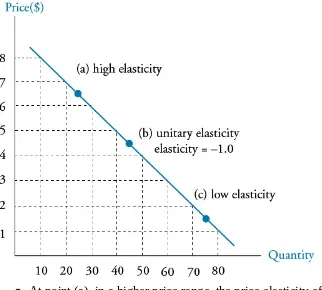
Figure 14.2: Price Elasticity Along a Linear Demand Curve

At point (a), in a higher price range, the price elasticity of demand is greater than at point (c) in a lower price range.

The elasticity at point (b) is –1.0; a 1% increase in price leads to a 1% decrease in quantity demanded. This is the point of greatest total revenue (P × Q), which is 4.50 × 45 = $202.50.

At prices less than $4.50 (inelastic range), total revenue will increase when price increases. The percentage decrease in quantity demanded will be less than the percentage increase in price.

At prices above $4.50 (elastic range), a price increase will decrease total revenue since the percentage decrease in quantity demanded will be greater than the percentage increase in price.

An important point to consider about the price and quantity combination for which price elasticity equals –1.0 (unit or unitary elasticity) is that total revenue (price × quantity) is maximized at that price. An increase in price moves us to the elastic region of the curve so that the percentage decrease in quantity demanded is greater than the

percentage increase in price, resulting in a decrease in total revenue. A decrease in price from the point of unitary elasticity moves us into the inelastic region of the curve so that the percentage decrease in price is more than the percentage increase in quantity

(17)

Income Elasticity of Demand

Recall that one of the independent variables in our example of a demand function for gasoline was income. The sensitivity of quantity demanded to a change in income is termed income elasticity. Holding other independent variables constant, we can

measure income elasticity as the ratio of the percentage change in quantity demanded to the percentage change in income.

For most goods, the sign of income elasticity is positive—an increase in income leads to an increase in quantity demanded. Goods for which this is the case are termed normal goods. For other goods, it may be the case that an increase in income leads to a decrease in quantity demanded. Goods for which this is true are termed inferior goods.

Cross Price Elasticity of Demand

Recall that some of the independent variables in a demand function are the prices of related goods (related in the sense that their prices affect the demand for the good in question). The ratio of the percentage change in the quantity demanded of a good to the percentage change in the price of a related good is termed the cross price elasticity of demand.

When an increase in the price of a related good increases demand for a good, the two goods are substitutes. If Bread A and Bread B are two brands of bread, considered good substitutes by many consumers, an increase in the price of one will lead consumers to purchase more of the other (substitute the other). When the cross price elasticity of demand is positive (price of one is up and quantity demanded for the other is up), we say those goods are substitutes.

When an increase in the price of a related good decreases demand for a good, the two goods are complements. If an increase in the price of automobiles (less automobiles purchased) leads to a decrease in the demand for gasoline, they are complements. Right shoes and left shoes are perfect complements for most of us and, as a result, shoes are priced by the pair. If they were priced separately, there is little doubt that an increase in the price of left shoes would decrease the quantity demanded of right shoes. Overall, the cross price elasticity of demand is more positive the better substitutes two goods are and more negative the better complements the two goods are.

Calculating Elasticities

The price elasticity of demand is defined as:

The term is the slope of a demand function that (for a linear demand function) takes the form:

quantity demanded = A + B × price

(18)

As an example, consider a demand function with A = 100 and B = –2, so that Q = 100 – 2P. The slope, , of this line is –2. The corresponding demand curve for this demand function is: P = 100 / 2 – Q / 2 = 50 – 1/2 Q. Therefore, given a demand curve, we can calculate the slope of the demand function as the reciprocal of slope term, –1/2, of the demand curve (i.e., the reciprocal of –1/2 is –2, the slope of the demand function).

EXAMPLE: Calculating price elasticity of demand

A demand function for gasoline is as follows: Q_Dgas = 138,500 – 12,500P_gas

Calculate the price elasticity at a gasoline price of $3 per gallon. Answer:

We can calculate the quantity demanded at a price of $3 per gallon as 138,500 – 12,500(3) = 101,000. Substituting 3 for P₀, 101,000 for Q₀, and –12,500 for , we can calculate the price elasticity of demand as:

For this demand function, at a price and quantity of $3 per gallon and 101,000 gallons, demand is inelastic.

The techniques for calculating the income elasticity of demand and the cross price elasticity of demand are the same, as illustrated in the following example. We assume values for all the independent variables, except the one of interest, then calculate elasticity for a given value of the variable of interest.

EXAMPLE: Calculating income elasticity and cross price elasticity

An individual has the following demand function for gasoline: Q_{D gas} = 15 – 3P_gas + 0.02I + 0.11P_BT – 0.008P_auto

where income and car price are measured in thousands, and the price of bus travel is measured in average dollars per 100 miles traveled.

Assuming the average automobile price is $22,000, income is $40,000, the price of bus travel is $25, and the price of gasoline is $3, calculate and interpret the income elasticity of gasoline demand and the cross price elasticity of gasoline demand with respect to the price of bus travel.

Answer:

Inserting the prices of gasoline, bus travel, and automobiles into our demand equation, we get: Q_{D gas} = 15 – 3(3) + 0.02(income in thousands) + 0.11(25) – 0.008(22)

and

Q_{D gas} = 8.6 + 0.02(income in thousands)

Our slope term on income is 0.02, and for an income of 40,000, Q_{D gas} = 9.4 gallons. The formula for the income elasticity of demand is:

(19)

Video covering this content is available online. This tells us that for these assumed values (at a single point on the demand curve), a 1% increase (decrease) in income will lead to an increase (decrease) of 0.085% in the quantity of gasoline demanded.

In order to calculate the cross price elasticity of demand for bus travel and gasoline, we construct a demand function with only the price of bus travel as an independent variable:

Q_{D gas} = 15 – 3P_gas + 0.02I + 0.11P_BT – 0.008P_auto Q_{D gas} = 15 – 3(3) + 0.02(40) + 0.11P_BT – 0.008(22) Q_{D gas} = 6.6 + 0.11P_BT

For a price of bus travel of $25, the quantity of gasoline demanded is: Q_{D gas} = 6.6 + 0.11P_BT

Q_{D gas} = 6.6 + 0.11(25) = 9.35 gallons

The cross price elasticity of the demand for gasoline with respect to the price of bus travel is:

As noted, gasoline and bus travel are substitutes, so the cross price elasticity of demand is positive. We can interpret this value to mean that, for our assumed values, a 1% change in the price of bus travel will lead to a 0.294% change in the quantity of gasoline demanded in the same direction, other things equal.

MODULE 14.2: DEMAND AND SUPPLY

LOS 14.b: Compare substitution and income effects.

CFA® Program Curriculum, Volume 2, page 18 When the price of Good X decreases, there is a substitution effect that shifts

consumption towards more of Good X. Because the total expenditure on the consumer’s original bundle of goods falls when the price of Good X falls, there is also an income effect. The income effect can be toward more or less consumption of Good X. This is the key point here: the substitution effect always acts to increase the consumption of a good that has fallen in price, while the income effect can either increase or decrease consumption of a good that has fallen in price.

Based on this analysis, we can describe three possible outcomes of a decrease in the price of Good X:

1. The substitution effect is positive, and the income effect is also positive— consumption of Good X will increase.

2. The substitution effect is positive, and the income effect is negative but smaller than the substitution effect—consumption of Good X will increase.

3. The substitution effect is positive, and the income effect is negative and larger than the substitution effect—consumption of Good X will decrease.

(20)

PROFESSOR’S NOTE

Candidates who are not already familiar with profit maximization based on a firm’s cost curves (e.g., average cost and marginal cost) and firm revenue (e.g., average revenue, total revenue, and marginal revenue) should study the material in the CFA curriculum prerequisite reading “Demand and Supply Analysis: The Firm” prior to their study of the following material.

Earlier, we defined normal goods and inferior goods in terms of their income elasticity of demand. A normal good is one for which the income effect is positive. An inferior good is one for which the income effect is negative.

A specific good may be an inferior good for some ranges of income and a normal good for other ranges of income. For a really poor person or population (e.g., underdeveloped country), an increase in income may lead to greater consumption of noodles or rice. Now, if incomes rise a bit (e.g., college student or developing country), more meat or seafood may become part of the diet. Over this range of incomes, noodles can be an inferior good and ground meat a normal good. If incomes rise to a higher range (e.g., graduated from college and got a job), the consumption of ground meat may fall (inferior) in favor of preferred cuts of meat (normal).

For many of us, commercial airline travel is a normal good. When our incomes rise, vacations are more likely to involve airline travel, be more frequent, and extend over longer distances so that airline travel is a normal good. For wealthy people (e.g., hedge fund manager), an increase in income may lead to travel by private jet and a decrease in the quantity of commercial airline travel demanded.

A Giffen good is an inferior good for which the negative income effect outweighs the positive substitution effect when price falls. A Giffen good is theoretical and would have an upward-sloping demand curve. At lower prices, a smaller quantity would be demanded as a result of the dominance of the income effect over the substitution effect. Note that the existence of a Giffen good is not ruled out by the axioms of the theory of consumer choice.

A Veblen good is one for which a higher price makes the good more desirable. The idea is that the consumer gets utility from being seen to consume a good that has high status (e.g., Gucci bag), and that a higher price for the good conveys more status and increases its utility. Such a good could conceivably have a positively sloped demand curve for some individuals over some range of prices. If such a good exists, there must be a limit to this process, or the price would rise without limit. Note that the existence of a Veblen good does violate the theory of consumer choice. If a Veblen good exists, it is not an inferior good, so both the substitution and income effects of a price increase are to decrease consumption of the good.

LOS 14.d: Describe the phenomenon of diminishing marginal returns.

(21)

Land—where the business facilities are located.

Labor—includes all workers from unskilled laborers to top management.

Capital—sometimes called physical capital or plant and equipment to distinguish it from financial capital. Refers to manufacturing facilities, equipment, and machinery.

Materials—refers to inputs into the productive process, including raw materials, such as iron ore or water, or manufactured inputs, such as wire or

microprocessors.

For economic analysis, we often consider only two inputs, capital and labor. The quantity of output that a firm can produce can be thought of as a function of the amounts of capital and labor employed. Such a function is called a production function.

If we consider a given amount of capital (a firm’s plant and equipment), we can examine the increase in production (increase in total product) that will result as we increase the amount of labor employed. The output with only one worker is considered the marginal product of the first unit of labor. The addition of a second worker will increase total product by the marginal product of the second worker. The marginal product of (additional output from) the second worker is likely greater than the marginal product of the first. This is true if we assume that two workers can produce more than twice as much output as one because of the benefits of teamwork or specialization of tasks. At this low range of labor input (remember, we are holding capital constant), we can say that the marginal product of labor is increasing.

As we continue to add additional workers to a fixed amount of capital, at some point, adding one more worker will increase total product by less than the addition of the previous worker, although total product continues to increase. When we reach the quantity of labor for which the additional output for each additional worker begins to decline, we have reached the point of diminishing marginal productivity of labor, or that labor has reached the point of diminishing marginal returns. Beyond this quantity of labor, the additional output from each additional worker continues to decline.

There is, theoretically, some quantity for labor for which the marginal product of labor is actually negative (i.e., the addition of one more worker actually decreases total output).

In Figure 14.3, we illustrate all three cases. For quantities of labor between zero and A, the marginal product of labor is increasing (slope is increasing). Beyond the inflection point in the production at quantity of labor A up to quantity B, the marginal product of labor is still positive but decreasing. The slope of the production function is positive but decreasing, and we are in a range of diminishing marginal productivity of labor. Beyond the quantity of labor B, adding additional workers decreases total output. The marginal product of labor in this range is negative, and the production function slopes downward.

(22)

LOS 14.e: Determine and interpret breakeven and shutdown points of production. CFA® Program Curriculum, Volume 2, page 28 In economics, we define the short run for a firm as the time period over which some factors of production are fixed. Typically, we assume that capital is fixed in the short run so that a firm cannot change its scale of operations (plant and equipment) over the short run. All factors of production (costs) are variable in the long run. The firm can let its leases expire and sell its equipment, thereby avoiding costs that are fixed in the short run.

Shutdown and Breakeven Under Perfect Competition

As a simple example of shutdown and breakeven analysis, consider a retail store with a 1-year lease (fixed cost) and one employee (quasi-fixed cost), so that variable costs are simply the store’s cost of merchandise. If the total sales (total revenue) just covers both fixed and variable costs, price equals both average revenue and average total cost, so we are at the breakeven output quantity, and economic profit equals zero.

During the period of the lease (the short run), as long as items are being sold for more than their variable cost, the store should continue to operate to minimize losses. If items are being sold for less than their average variable cost, losses would be reduced by shutting down the business in the short run.

In the long run, a firm should shut down if the price is less than average total cost, regardless of the relation between price and average variable cost.

(23)

above P₁, economic profit is positive, and at prices less than P₁, economic profit is negative (the firm has economic losses).

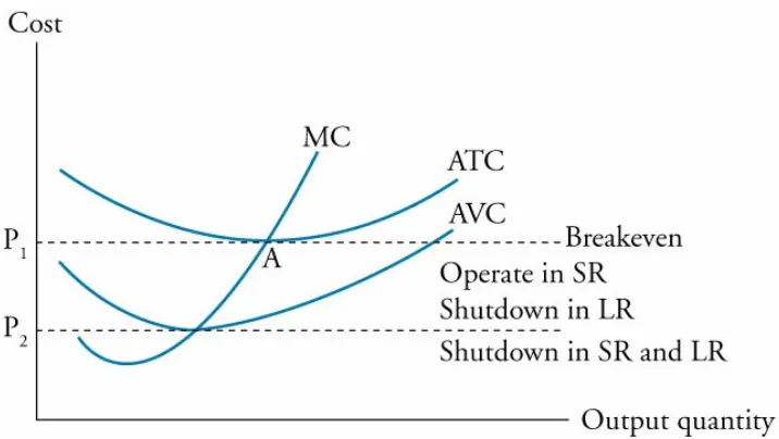
Figure 14.4: Shutdown and Breakeven

Because some costs are fixed in the short run, it will be better for the firm to continue production in the short run as long as average revenue is greater than average variable costs. At prices between P₁ and P₂ in Figure 14.4, the firm has losses, but the loss is less than the losses that would occur if all production were stopped. As long as total revenue is greater than total variable cost, at least some of the firm’s fixed costs are covered by continuing to produce and sell its product. If the firm were to shut down, losses would be equal to the fixed costs that still must be paid. As long as price is greater than average variable costs, the firm will minimize its losses in the short run by continuing in business.

If average revenue is less average variable cost, the firm’s losses are greater than its fixed costs, and it will minimize its losses by shutting down production in the short run. In this case (a price less than P2 in Figure 14.4), the loss from continuing to operate is greater than the loss (total fixed costs) if the firm is shut down.

In the long run, all costs are variable, so a firm can avoid its (short-run) fixed costs by shutting down. For this reason, if price is expected to remain below minimum average total cost (Point A in Figure 14.4) in the long run, the firm will shut down rather than continue to generate losses.

To sum up, if average revenue is less than average variable cost in the short run, the firm should shut down. This is its short-run shutdown point. If average revenue is greater than average variable cost in the short run, the firm should continue to operate, even if it has losses. In the long run, the firm should shut down if average revenue is less than average total cost. This is the long-run shutdown point. If average revenue is just equal to average total cost, total revenue is just equal to total (economic) cost, and this is the firm’s breakeven point.

(24)

If AR ≥ AVC, but AR < ATC, the firm should stay in the market in the short run but will exit the market in the long run.

If AR < AVC, the firm should shut down in the short run and exit the market in the long run.

Shutdown and Breakeven Under Imperfect

Competition

For price-searcher firms (those that face downward-sloping demand curves), we could compare average revenue to ATC and AVC, just as we did for price-taker firms, to identify shutdown and breakeven points. However, marginal revenue is no longer equal to price.

We can, however, still identify the conditions under which a firm is breaking even, should shut down in the short run, and should shut down in the long run in terms of total costs and total revenue. These conditions are:

TR = TC: break even.

TC > TR > TVC: firm should continue to operate in the short run but shut down in the long run.

TR < TVC: firm should shut down in the short run and the long run.

Because price does not equal marginal revenue for a firm in imperfect competition, analysis based on total costs and revenues is better suited for examining breakeven and shutdown points.

The previously described relations hold for both price-taker and price-searcher firms. We illustrate these relations in Figure 14.5 for a price-taker firm (TR increases at a constant rate with quantity). Total cost equals total revenue at the breakeven quantities Q_BE1 and Q_BE2. The quantity for which economic profit is maximized is shown as Q_max.

(25)

If the entire TC curve exceeds TR (i.e., no breakeven point), the firm will want to minimize the economic loss in the short run by operating at the quantity corresponding to the smallest (negative) value of TR – TC.

EXAMPLE: Short-run shutdown decision

For the last fiscal year, Legion Gaming reported total revenue of $700,000, total variable costs of $800,000, and total fixed costs of $400,000. Should the firm continue to operate in the short run? Answer:

The firm should shut down. Total revenue of $700,000 is less than total costs of $1,200,000 and also less than total variable costs of $800,000. By shutting down, the firm will lose an amount equal to fixed costs of $400,000. This is less than the loss of operating, which is TR – TC = $500,000.

EXAMPLE: Long-run shutdown decision

Suppose instead that Legion reported total revenue of $850,000. Should the firm continue to operate in the short run? Should it continue to operate in the long run?

Answer:

In the short run, TR > TVC, and the firm should continue operating. The firm should consider exiting the market in the long run, as TR is not sufficient to cover all of the fixed costs and variable costs.

(26)

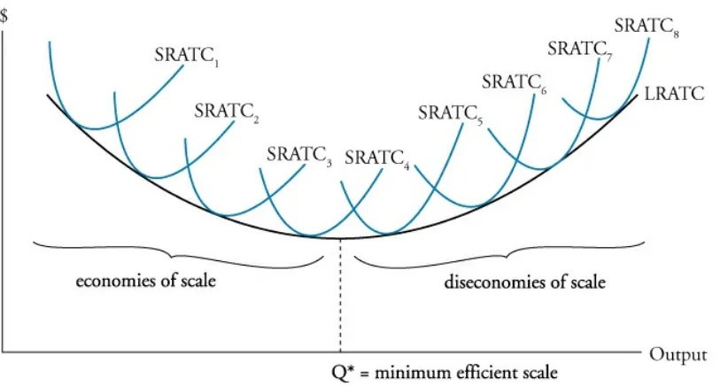
is drawn for many different plant sizes or scales of operation, each point along the curve represents the minimum ATC for a given plant size or scale of operations. In Figure 14.6, we show a firm’s LRATC curve along with short-run average total cost (SRATC) curves for many different plant sizes, with SRATC_n+1 representing a larger scale of operations than SRATC_n.

Figure 14.6: Economies and Diseconomies of Scale

We draw the LRATC curve as U-shaped. Average total costs first decrease with larger scale and eventually increase. The lowest point on the LRATC corresponds to the scale or plant size at which the average total cost of production is at a minimum. This scale is sometimes called the minimum efficient scale. Under perfect competition, firms must operate at minimum efficient scale in long-run equilibrium, and LRATC will equal the market price. Recall that under perfect competition, firms earn zero economic profit in long-run equilibrium. Firms that have chosen a different scale of operations with higher average total costs will have economic losses and must either leave the industry or change to minimum efficient scale.

The downward-sloping segment of the long-run average total cost curve presented in

Figure 14.6 indicates that economies of scale (or increasing returns to scale) are present. Economies of scale result from factors such as labor specialization, mass

production, and investment in more efficient equipment and technology. In addition, the firm may be able to negotiate lower input prices with suppliers as firm size increases and more resources are purchased. A firm operating with economies of scale can increase its competitiveness by expanding production and reducing costs.

The upward-sloping segment of the LRATC curve indicates that diseconomies of scale

are present. Diseconomies of scale may result as the increasing bureaucracy of larger firms leads to inefficiency, problems with motivating a larger workforce, and greater barriers to innovation and entrepreneurial activity. A firm operating under diseconomies of scale will want to decrease output and move back toward the minimum efficient scale. The U.S. auto industry is an example of an industry that has exhibited

(27)

There may be a relatively flat portion at the bottom of the LRATC curve that exhibits constant returns to scale. Over a range of constant returns to scale, costs are constant for the various plant sizes.

MODULE QUIZ 14.1, 14.2

To best evaluate your performance, enter your quiz answers online. 1. Total revenue is greatest in the part of a demand curve that is:

A. elastic B. inelastic C. unit elastic.

2. A demand function for air conditioners is given by:

QD_{air conditioner} = 10,000 – 2 P_{air conditioner} + 0.0004 income + 30 P_{electric fan} – 4 Pelectricity

At current average prices, an air conditioner costs 5,000 yen, a fan costs 200 yen, and electricity costs 1,000 yen. Average income is 4,000,000 yen. The income elasticity of demand for air conditioners is closest to:

A. 0.0004. B. 0.444. C. 40,000.

3. When the price of a good decreases, and an individual’s consumption of that good also decreases, it is most likely that the:

A. income effect and substitution effect are both negative.

B. substitution effect is negative and the income effect is positive. C. income effect is negative and the substitution effect is positive. 4. A good is classified as an inferior good if its:

A. income elasticity is negative. B. own-price elasticity is negative. C. cross-price elasticity is negative.

5. Increasing the amount of one productive input while keeping the amounts of other inputs constant results in diminishing marginal returns:

A. in all cases.

B. when it causes total output to decrease.

C. when the increase in total output becomes smaller.

6. A firm’s average revenue is greater than its average variable cost and less than its average total cost. If this situation is expected to persist, the firm should:

A. shut down in the short run and in the long run.

B. shut down in the short run but operate in the long run. C. operate in the short run but shut down in the long run.

7. If a firm’s long-run average total cost increases by 6% when output is increased by 6%, the firm is experiencing:

(28)

KEY CONCEPTS

LOS 14.a

Elasticity is measured as the ratio of the percentage change in one variable to a percentage change in another. Three elasticities related to a demand function are of interest:

|own price elasticity| > 1: demand is elastic |own price elasticity| < 1: demand is inelastic

cross price elasticity > 0: related good is a substitute cross price elasticity < 0: related good is a complement income elasticity < 0: good is an inferior good

income elasticity > 0: good is a normal good

LOS 14.b

When the price of a good decreases, the substitution effect leads a consumer to consume more of that good and less of goods for which prices have remained the same.

A decrease in the price of a good that a consumer purchases leaves her with unspent income (for the same combination of goods). The effect of this additional income on consumption of the good for which the price has decreased is termed the income effect.

LOS 14.c

For a normal good, the income effect of a price decrease is positive—income elasticity of demand is positive.

For an inferior good, the income effect of a price decrease is negative—income

elasticity of demand is negative. An increase in income reduces demand for an inferior good.

A Giffen good is an inferior good for which the negative income effect of a price decrease outweighs the positive substitution effect, so that a decrease (increase) in the good’s price has a net result of decreasing (increasing) the quantity consumed.

A Veblen good is also one for which an increase (decrease) in price results in an

(29)

LOS 14.d

Marginal returns refer to the additional output that can be produced by using one more unit of a productive input while holding the quantities of other inputs constant. Marginal returns may increase as the first units of an input are added, but as input quantities increase, they reach a point at which marginal returns begin to decrease. Inputs beyond this quantity are said to produce diminishing marginal returns.

LOS 14.e

Under perfect competition:

The breakeven quantity of production is the quantity for which price (P) = average total cost (ATC) and total revenue (TR) = total cost (TC).

The firm should shut down in the long run if P < ATC so that TR < TC. The firm should shut down in the short run (and the long run) if P < average variable cost (AVC) so that TR < total variable cost (TVC).

Under imperfect competition (firm faces downward sloping demand): Breakeven quantity is the quantity for which TR = TC.

The firm should shut down in the long run if TR < TC.

The firm should shut down in the short run (and the long run) if TR < TVC.

LOS 14.f

The long-run average total cost (LRATC) curve shows the minimum average total cost for each level of output assuming that the plant size (scale of the firm) can be adjusted. A downward-sloping segment of an LRATC curve indicates economies of scale

(30)

ANSWER KEY FOR MODULE QUIZZES

Module Quiz 14.1, 14.2

1. C Total revenue is maximized at the quantity at which own-price elasticity equals –1. (Module 14.1, LOS 14.a)

2. B Substituting current values for the independent variables other than income, the demand function becomes:

QD_{air conditioner} = 10,000 – 2(5,000) + 0.0004 income + 30(200) – 4(1,000)

= 0.0004 income + 2,000.

The slope of income is 0.0004, and for an income of 4,000,000 yen, QD = 3,600.

Income elasticity = I₀ / Q₀ × ∆Q / ∆I = 4,000,000 / 3,600 × 0.0004 = 0.444. (Module 14.1, LOS 14.a)

3. C The substitution effect of a price decrease is always positive, but the income effect can be either positive or negative. Consumption of a good will decrease when the price of that good decreases only if the income effect is both negative and greater than the substitution effect. (Module 14.2, LOS 14.b)

4. A An inferior good is one that has a negative income elasticity of demand. (Module 14.2, LOS 14.c)

5. C Productive inputs exhibit diminishing marginal returns at the level where an additional unit of input results in a smaller increase in output than the previous unit of input. (Module 14.2, LOS 14.d)

6. C If a firm is generating sufficient revenue to cover its variable costs and part of its fixed costs, it should continue to operate in the short run. If average revenue is likely to remain below average total costs in the long run, the firm should shut down. (Module 14.2, LOS 14.e)

(31)

Video covering this content is available online. The following is a review of the Economics (1) principles designed to address the learning outcome statements set forth by CFA Institute. Cross-Reference to CFA Institute Assigned Reading #15.

READING 15: THE FIRM AND MARKET

STRUCTURES

Study Session 4

EXAM FOCUS

This topic review covers four market structures: perfect competition, monopolistic competition, oligopoly, and monopoly. You need to be able to compare and contrast these structures in terms of numbers of firms, firm demand elasticity and pricing power, long-run economic profits, barriers to entry, and the amount of product differentiation and advertising. Finally, know the two quantitative concentration measures, their implications for market structure and pricing power, and their limitations in this regard. We will apply all of these concepts when we analyze industry competition and pricing power of companies in the Study Session on equity investments.

MODULE 15.1: PERFECT COMPETITION

LOS 15.a: Describe characteristics of perfect competition, monopolistic competition, oligopoly, and pure monopoly.

In this topic review, we examine four types of market structure: perfect competition, monopolistic competition, oligopoly, and monopoly. We can analyze where an industry falls along this spectrum by examining the following five factors:

1. Number of firms and their relative sizes.

2. Degree to which firms differentiate their products. 3. Bargaining power of firms with respect to pricing. 4. Barriers to entry into or exit from the industry.

5. Degree to which firms compete on factors other than price.

At one end of the spectrum is perfect competition, in which many firms produce identical products, and competition forces them all to sell at the market price. At the other extreme, we have monopoly, where only one firm is producing the product. In between are monopolistic competition (many sellers and differentiated products) and

(32)

basis of price. Firms face perfectly elastic (horizontal) demand curves at the price

determined in the market because no firm is large enough to affect the market price. The market for wheat in a region is a good approximation of such a market. Overall market supply and demand determine the price of wheat.

Monopolistic competition differs from perfect competition in that products are not identical. Each firm differentiates its product(s) from those of other firms through some combination of differences in product quality, product features, and marketing. The demand curve faced by each firm is downward sloping; while demand is elastic, it is not perfectly elastic. Prices are not identical because of perceived differences among

competing products, and barriers to entry are low. The market for toothpaste is a good example of monopolistic competition. Firms differentiate their products through features and marketing with claims of more attractiveness, whiter teeth, fresher breath, and even of actually cleaning your teeth and preventing decay. If the price of your personal favorite increases, you are not likely to immediately switch to another brand as under perfect competition. Some customers would switch in response to a 10% increase in price and some would not. This is why firm demand is downward sloping.

The most important characteristic of an oligopoly market is that there are only a few firms competing. In such a market, each firm must consider the actions and responses of other firms in setting price and business strategy. We say that such firms are

interdependent. While products are typically good substitutes for each other, they may be either quite similar or differentiated through features, branding, marketing, and quality. Barriers to entry are high, often because economies of scale in production or marketing lead to very large firms. Demand can be more or less elastic than for firms in monopolistic competition. The automobile market is dominated by a few very large firms and can be characterized as an oligopoly. The product and pricing decisions of Toyota certainly affect those of Ford and vice versa. Automobile makers compete based on price, but also through marketing, product features, and quality, which is often signaled strongly through brand name. The oil industry also has a few dominant firms but their products are very good substitutes for each other.

A monopoly market is characterized by a single seller of a product with no close

substitutes. This fact alone means that the firm faces a downward-sloping demand curve (the market demand curve) and has the power to choose the price at which it sells its product. High barriers to entry protect a monopoly producer from competition. One source of monopoly power is the protection offered by copyrights and patents. Another possible source of monopoly power is control over a resource specifically needed to produce the product. Most frequently, monopoly power is supported by government. A

natural monopoly refers to a situation where the average cost of production is falling over the relevant range of consumer demand. In this case, having two (or more)

(33)

information on buyers and sellers and the number of buyers who visit eBay essentially precluded others from establishing competing businesses. While it may have

competition to some degree, its market share is such that it has negatively sloped demand and a good deal of pricing power. Sometimes we refer to such companies as having a moat around them that protects them from competition. It is best to remember, however, that changes in technology and consumer tastes can, and usually do, reduce market power over time. Polaroid had a monopoly on instant photos for years, but the introduction of digital photography forced the firm into bankruptcy in 2001.

The table in Figure 15.1 shows the key features of each market structure.

Figure 15.1: Characteristics of Market Structures

LOS 15.b: Explain relationships between price, marginal revenue, marginal cost, economic profit, and the elasticity of demand under each market structure.

LOS 15.d: Describe and determine the optimal price and output for firms under each market structure.

LOS 15.e: Explain factors affecting long-run equilibrium under each market structure.

PROFESSOR’S NOTE

We cover these LOS together and slightly out of curriculum order so that we can present the complete analysis of each market structure to better help candidates understand the

economics of each type of market structure.

Producer firms in perfect competition have no influence over market price. Market supply and demand determine price. As illustrated in Figure 15.2, the individual firm’s demand schedule is perfectly elastic (horizontal).

(34)

In a perfectly competitive market, a firm will continue to expand production until marginal revenue (MR) equals marginal cost (MC). Marginal revenue is the increase in total revenue from selling one more unit of a good or service. For a price taker, marginal revenue is simply the price because all additional units are assumed to be sold at the same (market) price. In pure competition, a firm’s marginal revenue is equal to the market price, and a firm’s MR curve, presented in Figure 15.3, is identical to its demand curve. A profit maximizing firm will produce the quantity, Q*, when MC = MR.

Figure 15.3: Profit Maximizing Output For A Price Taker

All firms maximize (economic) profit by producing and selling the quantity for which marginal revenue equals marginal cost. For a firm in a perfectly competitive market, this is the same as producing and selling the quantity for which marginal cost equals (market) price. Economic profit equals total revenues less the opportunity cost of production, which includes the cost of a normal return to all factors of production, including invested capital.

Panel (a) of Figure 15.4 illustrates that in the short run, economic profit is maximized at the quantity for which marginal revenue = marginal cost. As shown in Panel (b), profit maximization also occurs when total revenue exceeds total cost by the maximum amount.

(35)

An economic loss occurs on any units for which marginal revenue is less than marginal cost. At any output above the quantity where MR = MC, the firm will be generating losses on its marginal production and will maximize profits by reducing output to where MR = MC.

In a perfectly competitive market, firms will not earn economic profits for any

significant period of time. The assumption is that new firms (with average and marginal cost curves identical to those of existing firms) will enter the industry to earn economic profits, increasing market supply and eventually reducing market price so that it just equals firms’ average total cost (ATC). In equilibrium, each firm is producing the quantity for which P = MR = MC = ATC, so that no firm earns economic profits and each firm is producing the quantity for which ATC is a minimum (the quantity for which ATC = MC). This equilibrium situation is illustrated in Figure 15.5.

Figure 15.5: Equilibrium in a Perfectly Competitive Market

(36)

continuing to operate, its losses will be greater than its fixed costs. In this case, the firm will shut down (zero output) and lay off its workers. This will limit its losses to its fixed costs (e.g., its building lease and debt payments). If the firm does not believe price will ever exceed ATC in the future, going out of business is the only way to eliminate fixed costs.

Figure 15.6: Short-Run Loss

The long-run equilibrium output level for perfectly competitive firms is where MR = MC = ATC, which is where ATC is at a minimum. At this output, economic profit is zero and only a normal return is realized.

Recall that price takers should produce where P = MC. Referring to Panel (a) in Figure 15.7, a firm will shut down at a price below P₁. Between P₁ and P₂, a firm will continue to operate in the short run. At P₂, the firm is earning a normal profit—economic profit equals zero. At prices above P₂, a firm is making economic profits and will expand its production along the MC line. Thus, the short-run supply curve for a firm is its MC line above the average variable cost curve, AVC. The supply curve shown in Panel (b) is the short-run market supply curve, which is the horizontal sum (add up the

quantities from all firms at each price) of the MC curves for all firms in a given industry. Because firms will supply more units at higher prices, the short-run market supply curve slopes upward to the right.

(37)

Changes in Demand, Entry and Exit, and Changes in

Plant Size

In the short run, an increase in market demand (a shift of the market demand curve to the right) will increase both equilibrium price and quantity, while a decrease in market demand will reduce both equilibrium price and quantity. The change in equilibrium price will change the (horizontal) demand curve faced by each individual firm and the profit-maximizing output of a firm. These effects for an increase in demand are

illustrated in Figure 15.8. An increase in market demand from D₁ to D₂ increases the short-run equilibrium price from P₁ to P₂ and equilibrium output from Q₁ to Q₂. In Panel (b) of Figure 15.8, we see the short-run effect of the increased market price on the output of an individual firm. The higher price leads to a greater profit-maximizing output, Q2 Firm. At the higher output level, a firm will earn an economic profit in the short run. In the long run, some firms will increase their scale of operations in response to the increase in demand, and new firms will likely enter the industry. In response to a decrease in demand, the short-run equilibrium price and quantity will fall, and in the long run, firms will decrease their scale of operations or exit the market.

Figure 15.8: Short-Run Adjustment to an Increase in Demand Under Perfect Competition

A firm’s long-run adjustment to a shift in industry demand and the resulting change in price may be either to alter the size of its plant or leave the market entirely. The

marketplace abounds with examples of firms that have increased their plant sizes (or added additional production facilities) to increase output in response to increasing market demand. Other firms, such as Ford and GM, have decreased plant size to reduce economic losses. This strategy is commonly referred to as downsizing.

If an industry is characterized by firms earning economic profits, new firms will enter the market. This will cause industry supply to increase (the industry supply curve shifts downward and to the right), increasing equilibrium output and decreasing equilibrium price. Even though industry output increases, however, individual firms will produce less because as price falls, each individual firm will move down its own supply curve. The end result is that a firm’s total revenue and economic profit will decrease.

(38)

production at the higher market price. This will cause total revenues to increase, reducing any economic losses the remaining firms had been experiencing.

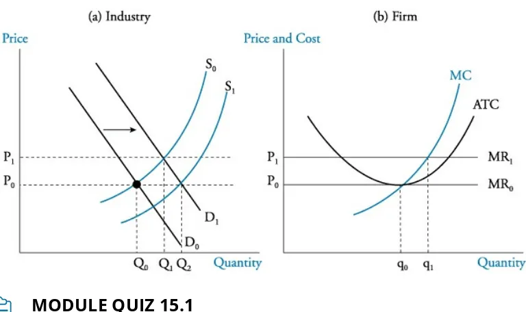
A permanent change in demand leads to the entry of firms to, or exit of firms from, an industry. Let’s consider the permanent increase in demand illustrated in Figure 15.9. The initial long-run industry equilibrium condition shown in Panel (a) is at the

intersection of demand curve D₀ and supply curve S₀, at price P₀ and quantity Q₀. As indicated in Panel (b) of Figure 15.9, at the market price of P₀ each firm will produce q₀. At this price and output, each firm earns a normal profit, and economic profit is zero. That is, MC = MR = P, and ATC is at its minimum. Now, suppose industry

demand permanently increases such that the industry demand curve in Panel (a) shifts to D₁. The new market price will be P₁ and industry output will increase to Q₁. At the new price P1, existing firms will produce q1 and realize an economic profit because P1 > ATC. Positive economic profits will cause new firms to enter the market. As these new firms increase total industry supply, the industry supply curve will gradually shift to S₁, and the market price will decline back to P₀. At the market price of P₀, the industry will now produce Q2, with an increased number of firms in the industry, each producing at the original quantity, q0. The individual firms will no longer enjoy an economic profit because ATC = P₀ at q₀.

Figure 15.9: Effects of a Permanent Increase in Demand

MODULE QUIZ 15.1

To best evaluate your performance, enter your quiz answers online.

1. When a firm operates under conditions of pure competition, marginal revenue always equals:

A. price.

B. average cost. C. marginal cost.

(39)

Video covering this content is available online. A. Oligopoly or monopoly.

B. Perfect competition only.

C. Perfect competition or monopolistic competition. 3. In a purely competitive market, economic losses indicate that:

A. price is below average total costs.

B. collusion is occurring in the market place. C. firms need to expand output to reduce costs.

4. A purely competitive firm will tend to expand its output so long as: A. marginal revenue is positive.

B. marginal revenue is greater than price. C. market price is greater than marginal cost.

5. A firm is likely to operate in the short run as long as price is at least as great as: A. marginal cost.

B. average total cost. C. average variable cost.

MODULE 15.2: MONOPOLISTIC

COMPETITION

Monopolistic competition has the following market characteristics: A large number of independent sellers: (1) Each firm has a

relatively small market share, so no individual firm has any significant power over price. (2) Firms need only pay attention to average market price, not the price of individual competitors. (3) There are too many firms in the industry for collusion (price fixing) to be possible.

Differentiated products: Each producer has a product that is slightly different from its competitors (at least in the minds of consumers). The competing products are close substitutes for one another.

Firms compete on price, quality, and marketing as a result of product

differentiation. Quality is a significant product-differentiating characteristic. Price and output can be set by firms because they face downward-sloping demand curves, but there is usually a strong correlation between quality and the price that firms can charge. Marketing is a must to inform the market about a product’s differentiating characteristics.

Low barriers to entry so that firms are free to enter and exit the market. If firms in the industry are earning economic profits, new firms can be expected to enter the industry.

Firms in monopolistic competition face downward-sloping demand curves (they are price searchers). Their demand curves are highly elastic because competing products are perceived by consumers as close substitutes. Think about the market for toothpaste. All toothpaste is quite similar, but differentiation occurs due to taste preferences, influential advertising, and the reputation of the seller.

(40)

competition maximize economic profits by producing where marginal revenue (MR) equals marginal cost (MC), and by charging the price for that quantity from the demand curve, D. Here the firm earns positive economic profits because price, P*, exceeds average total cost, ATC*. Due to low barriers to entry, competitors will enter the market in pursuit of these economic profits.

Figure 15.10: Short-Run and Long-Run Output Under Monopolistic Competition

Panel (b) of Figure 15.10 illustrates long-run equilibrium for a representative firm after new firms have entered the market. As indicated, the entry of new firms shifts the demand curve faced by each individual firm down to the point where price equals average total cost (P* = ATC*), such that economic profit is zero. At this point, there is no longer an incentive for new firms to enter the market, and long-run equilibrium is established. The firm in monopolistic competition continues to produce at the quantity where MR = MC but no longer earns positive economic profits.

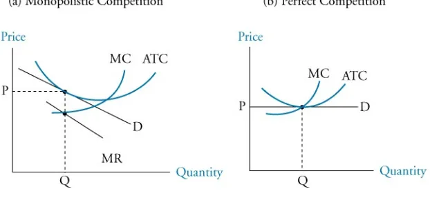
Figure 15.11 illustrates the differences between long-run equilibrium in markets with monopolistic competition and markets with perfect competition. Note that with

monopolistic competition, price is greater than marginal cost (i.e., producers can realize a markup), average total cost is not at a minimum for the quantity produced

(suggesting excess capacity, or an inefficient scale of production), and the price is slightly higher than under perfect competition. The point to consider here, however, is that perfect competition is characterized by no product differentiation. The question of the efficiency of monopolistic competition becomes, “Is there an economically efficient amount of product differentiation?”

(41)

In a world with only one brand of toothpaste, clearly average production costs would be lower. That fact alone probably does not mean that a world with only one brand/type of toothpaste would be a better world. While product differentiation has costs, it also has benefits to consumers.

Consumers definitely benefit from brand name promotion and advertising because they receive information about the nature of a product. This often enables consumers to make better purchasing decisions. Convincing consumers that a particular brand of deodorant will actually increase their confidence in a business meeting or make them more

attractive to the opposite sex is not easy or inexpensive. Whether the perception of increased confidence or attractiveness from using a particular product is worth the additional cost of advertising is a question probably better left to consumers of the products. Some would argue that the increased cost of advertising and sales is not justified by the benefits of these activities.

Product innovation is a necessary activity as firms in monopolistic competition pursue economic profits. Firms that bring new and innovative products to the market are

confronted with less-elastic demand curves, enabling them to increase price and earn economic profits. However, close substitutes and imitations will eventually erode the initial economic profit from an innovative product. Thus, firms in monopolistic

competition must continually look for innovative product features that will make their products relatively more desirable to some consumers than those of the competition. Innovation does not come without costs. The costs of product innovation must be weighed against the extra revenue that it produces. A firm is considered to be spending the optimal amount on innovation when the marginal cost of (additional) innovation just equals the marginal revenue (marginal benefit) of additional innovation.

Advertising expenses are high for firms in monopolistic competition. This is to inform consumers about the unique features of their products and to create or increase a

perception of differences between products that are actually quite similar. We just note here that advertising costs for firms in monopolistic competition are greater than those for firms in perfect competition and those that are monopolies.

As you might expect, advertising costs increase the average total cost curve for a firm in monopolistic competition. The increase to average total cost attributable to advertising decreases as output increases, because more fixed advertising dollars are being averaged over a larger quantity. In fact, if advertising leads to enough of an increase in output (sales), it can actually decrease a firm’s average total cost.

Brand names provide information to consumers by providing them with signals about the quality of the branded product. Many firms spend a significant portion of their advertising budget on brand name promotion. Seeing the brand name BMW on an automobile likely tells a consumer more about the quality of a newly introduced automobile than an inspection of the vehicle itself would reveal. At the same time, the reputation BMW has for high quality is so valuable that the firm has an added incentive not to damage it by producing vehicles of low quality.

MODULE QUIZ 15.2

(42)

Video covering this content is available online. 1. The demand for products from monopolistic competitors is relatively elastic due

to:

A. high barriers to entry.

B. the availability of many close substitutes. C. the availability of many complementary goods.

2. Compared to a perfectly competitive industry, in an industry characterized by monopolistic competition:

A. both price and quantity are likely to be lower.

B. price is likely to be higher and quantity is likely to be lower. C. quantity is likely to be higher and price is likely to be lower.

3. A firm will most likely maximize profits at the quantity of output for which: A. price equals marginal cost.

B. price equals marginal revenue.

C. marginal cost equals marginal revenue.

MODULE 15.3: OLIGOPOLY

Compared to monopolistic competition, an oligopoly market has higher barriers to entry and fewer firms. The other key difference is that the firms are interdependent, so a price change by one firm can be expected

to be met by a price change by its competitors. This means that the actions of another firm will directly affect a given firm’s demand curve for the product. Given this complicating fact, models of oligopoly pricing and profits must make a number of important assumptions. In the following, we describe four of these models and their implications for price and quantity:

1. Kinked demand curve model. 2. Cournot duopoly model.

3. Nash equilibrium model (prisoner’s dilemma). 4. Stackelberg dominant firm model.

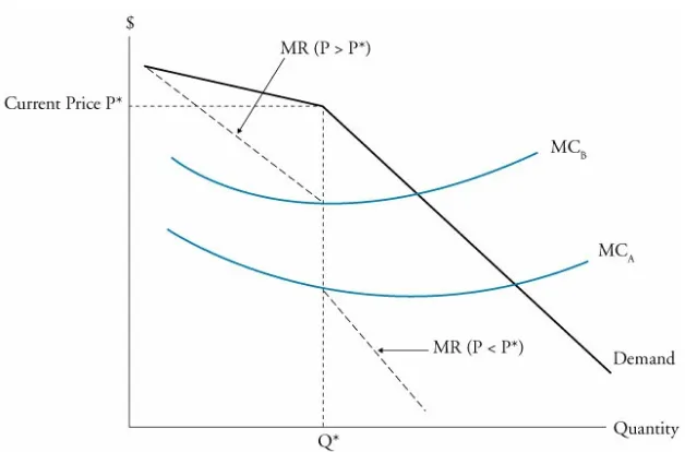
One traditional model of oligopoly, the kinked demand curve model, is based on the assumption that an increase in a firm’s product price will not be followed by its

competitors, but a decrease in price will. According to the kinked demand curve model, each firm believes that it faces a demand curve that is more elastic (flatter) above a given price (the kink in the demand curve) than it is below the given price. The kinked demand curve model is illustrated in Figure 15.12. The kink price is at price P_K, where a firm produces Q₀. A firm believes that if it raises its price above P₀, its competitors will remain at P0, and it will lose market share because it has the highest price. Above P₀, the demand curve is considered to be relatively elastic, where a small price increase will result in a large decrease in demand. On the other hand, if a firm decreases its price below P₀, other firms will match the price cut, and all firms will experience a relatively small increase in sales relative to any price reduction. Therefore, Q0 is the profit-maximizing level of output.

(43)

It is worth noting that with a kink in the market demand curve, we also get a gap in the associated marginal revenue curve, as shown in Figure 15.13. For any firm with a marginal cost curve passing through this gap, the price at which the kink is located is the firm’s profit maximizing price.

Figure 15.13: Gap in Marginal Revenue Curve

A shortcoming of the kinked demand curve model of oligopoly is that in spite of its intuitive appeal, it is incomplete because what determines the market price (where the kink is located) is outside the scope of the model.