Python
®
Programming
for Teens
Kenneth A. Lambert
Cengage Learning PTR
Python®Programming for Teens Kenneth A. Lambert
Publisher and General Manager, Cengage Learning PTR:Stacy L. Hiquet
Associate Director of Marketing:
Senior Product Manager:Mitzi Koontz
Project/Copy Editor:Karen A. Gill
Technical Reviewer:Zach Scott
Interior Layout Tech:MPS Limited
Cover Designer:Mike Tanamachi
Indexer:Sharon Shock
Proofreader:Gene Redding
©2015Cengage Learning PTR.
CENGAGE and CENGAGE LEARNING are registered trademarks of Cengage Learning, Inc., within the United States and certain other jurisdictions.
ALL RIGHTS RESERVED. No part of this work covered by the copyright herein may be reproduced, transmitted, stored, or used in any form or by any means graphic, electronic, or mechanical, including but not limited to photocopying, recording, scanning, digitizing, taping, Web distribution, information networks, or information storage and retrieval systems, except as permitted under Section107or108of the1976United States Copyright
Act, without the prior written permission of the publisher.
For product information and technology assistance, contact us at
Cengage Learning Customer & Sales Support,1-800-354-9706. For permission to use material from this text or product, submit all
requests online atcengage.com/permissions. Further permissions questions can be emailed to
Python is a registered trademark of the Python Software Foundation.
All other trademarks are the property of their respective owners.
All images © Cengage Learning unless otherwise noted.
Library of Congress Control Number:2014939193
ISBN-13:978-1-305-27195-1
Cengage Learning is a leading provider of customized learning solutions with office locations around the globe, including Singapore, the United Kingdom, Australia, Mexico, Brazil, and Japan. Locate your local office at:
international.cengage.com/region.
Cengage Learning products are represented in Canada by Nelson Education, Ltd.
For your lifelong learning solutions, visitcengageptr.com. Visit our corporate website atcengage.com.
Printed in the United States of America 1 2 3 4 5 6 7 16 15 14
To my wife Carolyn, with much gratitude. Kenneth A. Lambert
Acknowledgments
I would like to thank my friend Martin Osborne for many years of advice, friendly criticism, and encouragement on several of my book projects.
About the Author
Kenneth A. Lambertis a professor of computer science and the chair of that department at Washington and Lee University. He has taught introductory programming courses for 29 years and has been an active researcher in computer science education. Lambert has authored or coauthored 25 textbooks, including a series of introductory C++ textbooks with Douglas Nance and Thomas Naps, a series of introductory Java textbooks with Martin Osborne, and a series of introductory Python textbooks. His most recent textbook isFundamentals of Python: Data Structures.
Contents
Introduction . . . xiii
Chapter 1 Getting Started with Python . . . 1
Taking Care of Preliminaries . . . 1
Downloading and Installing Python . . . .1
Launching and Working in the IDLE Shell . . . .2
Obtaining Python Help. . . .3
Working with Numbers . . . 4
Using Arithmetic. . . .4
Working with Variables and Assignment . . . .6
Using Functions. . . .9
Using the math Module . . . .9
Detecting Errors . . . 11
Working with Strings . . . 12
String Literals . . . 12
The len, str, int, and float Functions . . . 14
Input and Output Functions. . . 15
Indexing, Slicing, and Concatenation . . . 16
String Methods . . . 18
Working with Lists . . . 19
List Literals and Operators . . . 19
List Methods . . . 20
Lists from Other Sequences . . . 22
Working with Dictionaries . . . 25
Dictionary Literals. . . 25
Dictionary Methods and Operators . . . 26
Summary . . . 27
Exercises . . . 29
Chapter 2 Getting Started with Turtle Graphics . . . 31
Looking at the Turtle and Its World . . . 31
Using Basic Movement Operations . . . 34
Moving and Changing Direction . . . 35
Drawing a Square . . . 36
Drawing an Equilateral Triangle . . . 38
Undoing, Clearing, and Resetting . . . 39
Setting and Examining the Turtle’s State . . . 40
The Pen Size . . . 40
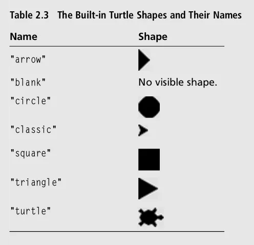
The Shape . . . 40
The Speed . . . 42
Other Information About the Turtle’s State . . . 42
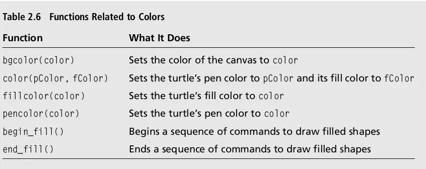
Working with Colors . . . 43
The Pen Color and the Background Color . . . 43
How Computers Represent Colors . . . 43
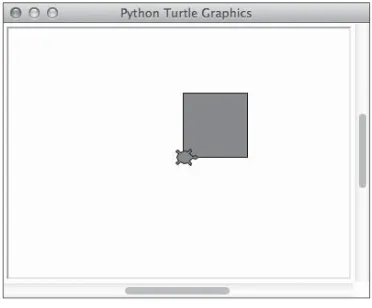
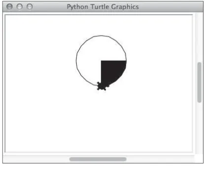
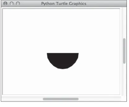
Filled Shapes . . . 45
Drawing Circles . . . 46
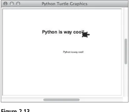
Drawing Text . . . 48
Using the Turtle’s Window and Canvas . . . 49
Using a Configuration File . . . 51
Summary . . . 51
Exercises . . . 52
Chapter 3 Control Structures: Sequencing, Iteration, and Selection . . . 55
Repeating a Sequence of Statements: Iteration . . . 56
The for Loop . . . 56
Nested Loops . . . 57
How the range Function Works with a for Loop . . . 58
Loops with Strings, Lists, and Dictionaries. . . 59
Asking Questions: Boolean Expressions. . . 60
Boolean Values . . . 61
Comparisons . . . 61
Making Choices: Selection Statements . . . 63
The One-Way if Statement . . . 63
The Two-Way if Statement . . . 65
Probable Options with random.randint . . . 66
The Multiway if Statement . . . 67
Using Selection to Control Iteration . . . 68
The while Loop . . . 69
Random Walks in Turtle Graphics . . . 70
Summary . . . 73
Exercises . . . 74
Chapter 4 Composing, Saving, and Running Programs. . . 75
Exploring the Program Development Process . . . 75
Composing a Program . . . 77
Program Edits . . . 77
Program Structure . . . 78
Docstrings and End-of-Line Comments . . . 79
import Statements . . . 79
The main Function . . . 79
The if main ==“__main__”Idiom . . . 80
The mainloop Function . . . 81
Running a Program . . . 81
Using a Turtle Graphics Configuration File . . . 81
Running a Program from an IDLE Window . . . 82
Running a Program from a Terminal Window . . . 83
Using the sys Module and Command-Line Arguments. . . 83
Looking Behind the Scenes: How Python Runs Programs . . . 85
Computer Hardware. . . 86
Computer Software . . . 88
Summary . . . 90
Exercises . . . 91
Chapter 5 Defining Functions . . . 93
Basic Elements of Function Definitions . . . 94
Circles and Squares . . . 94
Docstrings . . . 95
The return Statement. . . 96
Testing Functions in a Program . . . 97
Chapter 7 Recursion . . . 135
Recursive Design . . . 135
Top-Down Design . . . 135
Recursive Function Design . . . 137
Recursive Function Call Tracing . . . 139
Recursive Functions and Loops. . . 140
Infinite Recursion . . . 142
Sequential Search of a List . . . 143
Binary Search of a List . . . 145
Recursive Patterns in Art: Abstract Painting . . . 147
Design of the Program . . . 148
Performance Tracking . . . 148
The drawRectangle Function . . . 149
The mondrian Function . . . 149
The main Function . . . 151
The tracer and update Functions . . . 152
Recursive Patterns in Nature: Fractals . . . 153
What the Program Does. . . 155
Design of the Program . . . 155
Code for the Program . . . 156
Summary . . . 157
Exercises . . . 158
Chapter 8 Objects and Classes . . . 159
Objects, Methods, and Classes in Turtle Graphics . . . 160
The Turtle Class and Its Methods . . . 160
A Random Walk with Several Turtles . . . 161
A New Class: RegularPolygon . . . 162
Design: Determine the Attributes . . . 163
Design: Determine the Behavior . . . 164
Implementation: The Structure of a Class Definition . . . 166
Implementation: The __init__ Method . . . 168
Implementation: Showing and Hiding . . . 169
Implementation: Getting and Setting . . . 170
Implementation: Translation, Scaling, and Rotation . . . 171
Inheritance: Squares and Hexagons as Subclasses. . . 171
New Class: Menu Item . . . 172
Design: Determine the Attributes and Behavior. . . 173
Response to User Events, Revisited . . . 176
Whose Click Is It Anyway? . . . 176
A Grid Class for the Game of Tic-Tac-Toe . . . 179
Modeling a Grid . . . 179
Defining a Class for a Tic-Tac-Toe Grid . . . 181
Using Class Variables . . . 182
Stretching the Shape of a Turtle . . . 183
Making a Move. . . 183
Defining a Class for the Grid . . . 184
Laying Out the Grid . . . 184
Defining Methods for the Game Logic . . . 185
Coding the Main Application Module . . . 186
Summary . . . 187
Exercises . . . 188
Chapter 9 Animations . . . 189
Animating the Turtle with a Timer . . . 189
Using the ontimer Function . . . 190
Scheduling Actions at Regular Intervals . . . 190
Animating Many Turtles. . . 193
What Is an Animated Turtle? . . . 193
Using an Animated Turtle in a Shell Session . . . 195
Defining the AnimatedTurtle Class . . . 195
Sleepy and Speedy as Animated Turtles . . . 197
Creating Custom Turtle Shapes . . . 199
Creating Simple Shapes . . . 199
Creating Compound Shapes. . . 202
Summary . . . 203
Exercises . . . 204
Appendix A Turtle Graphics Commands . . . 205
Turtle Functions . . . 205
Turtle Motion . . . 205
Pen Control . . . 207
Turtle State . . . 209
Event Handling . . . 210
Functions Related to the Window and Canvas . . . 211
Window Functions . . . 211
Appendix B Solutions to Exercises . . . 213
Exercise Solutions for Chapter 1 . . . 213
Exercise 1. . . 213
Exercise 2. . . 213
Exercise Solutions for Chapter 2 . . . 213
Exercise 1. . . 213
Exercise 2. . . 214
Exercise Solutions for Chapter 3 . . . 216
Exercise 1. . . 216
Exercise 2. . . 216
Exercise Solutions for Chapter 4 . . . 216
Exercise 1. . . 216
Exercise 2. . . 217
Exercise Solutions for Chapter 5 . . . 218
Exercise 1. . . 218
Exercise 2. . . 218
Exercise Solutions for Chapter 6 . . . 219
Exercise 1. . . 219
Exercise 2. . . 221
Exercise Solutions for Chapter 7 . . . 222
Exercise 1. . . 222
Exercise 2. . . 222
Exercise Solutions for Chapter 8 . . . 224
Exercise 1. . . 224
Exercise 2. . . 227
Exercise Solutions for Chapter 9 . . . 229
Exercise 1. . . 229
Exercise 2. . . 231
Introduction
Welcome toPython Programming for Teens. Whether you’re under 20 or just a teenager at heart, this book will introduce you to computer programming. You can use it in a class-room or on your own. The only assumption is that you know how to use a modern com-puter system with a keyboard, screen, and mouse.
To make your learning experience fun and interesting, you will write programs that draw pictures on the screen and allow you to interact with them by using the mouse. Along the way, you will learn the basic principles of program design and problem solving with com-puters. You will then be able to apply these ideas and techniques to solve problems in almost any area of study. But most of all, you will experience the joy of building things that workand look great!
Why Python?
Computer technology and applications have become increasingly more sophisticated over the past several decades, and so has the computer science curriculum, especially at the introductory level. Today’s students learn a bit of programming and problem solving and are then expected to move quickly into topics like software development, complexity analysis, and data structures that, 20 years ago, were reserved for advanced courses. In addition, the ascent of object-oriented programming as a dominant method has led instructors and textbook authors to bring powerful, industrial-strength programming lan-guages such as C++ and Java into the introductory curriculum. As a result, instead of experiencing the rewards and excitement of computer programming, beginning students
often become overwhelmed by the combined tasks of mastering advanced concepts and learning the syntax of a programming language.
This book uses the Python programming language as a way of making the learning expe-rience manageable and attractive for students and instructors alike. Python offers the fol-lowing pedagogical benefits:
n Python has simple, conventional syntax. Its statements are close to those of ordinary English, and its expressions use the conventional notation found in algebra. Thus, beginners can spend less time learning the syntax of a programming language and more time learning to solve interesting problems.
n Python has safe semantics. Any expression or statement whose meaning violates the definition of the language produces an error message.
n Python scales well. It is easy for beginners to write simple programs. Python also includes all the advanced features of a modern programming language, such as support for data structures and object-oriented software development, for use when they become necessary.
n Python is highly interactive. Expressions and statements can be entered at an interpreter’s prompts to allow the programmer to try out experimental code and receive immediate feedback. Longer code segments can then be composed and saved in script files to be loaded and run as modules or standalone applications.
n Python is general purpose. In today’s context, this means that the language includes resources for contemporary applications, including media computing and networks.
n Python is free and is in widespread use in the industry. Students can download it to
run on a variety of devices. There is a large Python user community, and expertise in Python programming has great resume value.
Organization of the Book
The approach in this book is easygoing, with each new concept introduced only when you need it.
Chapter 1,“Getting Started with Python,” advises you how to download, install, and start the Python programming software used in this book. You try out simple program com-mands and become acquainted with the basic features of the Python language that you will use throughout the book.
Chapter 2, “Getting Started with Turtle Graphics,” introduces the basic commands for turtle graphics. You learn to draw pictures with a set of simple commands. Along the way, you discover a thing or two about colors and two-dimensional geometry.
Chapter 3,“Control Structures: Sequencing, Iteration, and Selection,” covers the program commands that allow the computer to make choices and perform repetitive tasks.
Chapters 4, “Composing, Saving, and Running Programs,” shows you how to save your programs in files, so you can give them to others or work on them another day. You learn how to organize a program like an essay, so it is easy for you and others to read, understand, and edit. You also learn a bit about how the computer is able to read, under-stand, and run a program.
Chapter 5,“Defining Functions,”introduces an important design feature: the function. By organizing your programs with functions, you can simplify complex tasks and eliminate unnecessary duplications in your code.
Chapter 6, “User Interaction with the Mouse and the Keyboard,” covers features that allow people to interact with your programs. You learn program commands for respond-ing to mouse and keyboard events, as well as pop-up dialogs that can take information from your programs’ users.
Chapter 7,“Recursion,”teaches you about another important design strategy called recur-sion. You write some recursive functions that generate computer art and fractal images.
Chapter 8,“Objects and Classes,”offers a beginner’s guide to the use of objects and classes in programming. You learn how to define new types of objects, such as menu items for choosing colors and grids for board games, and use them in interesting programs.
Chapter 9,“Animations,”concludes the book with a brief introduction to animations. You discover how to get images to move independently and interact in interesting ways.
Two appendixes follow the last chapter. Appendix A, “Turtle Graphics Commands,” provides a reference for the set of turtle graphics commands introduced in the book.
Each chapter includes a set of two programming exercises that build on concepts and examples introduced earlier in that chapter. You can find the answers to these exercises in Appendix B,“Solutions to Exercises.”
Companion Website Downloads
You may download the companion website files from www.cengageptr.com/downloads. These files include the example programs discussed in the book and the solutions to the exercises.
A Brief History of Computing
Before you jump ahead to programming, you might want to peek at some context. The following table summarizes some of the major developments in the history of computing. The discussion that follows provides more details about these developments.
Approximate Date Major Developments
Before 1800 Mathematicians develop and use algorithms Abacus used as a calculating aide
First mechanical calculators built by Leibniz and Pascal
1800–1930 Jacquard’s loom
Babbage’s Analytical Engine Boole’s system of logic
Hollerith’s punch card machine
1930s Turing publishes results on computability
Shannon’s theory of information and digital switching
1940s First electronic digital computers
1950s First symbolic programming languages
Transistors make computers smaller, faster, more durable, less expensive
Emergence of data-processing applications
1960–1975 Integrated circuits accelerate the miniaturization of computer hardware
First minicomputers
Time-sharing operating systems
Interactive user interfaces with keyboards and monitors Proliferation of high-level programming languages
1975–1990 First microcomputers and mass-produced personal computers Graphical user interfaces become widespread
Networks and the Internet
1990–2000 Optical storage (CDs, DVDs) Laptop computers
Multimedia applications (music, photography, video) Computer-assisted manufacturing, retail, and finance World Wide Web and e-commerce
2000–present Embedded computing (cars, appliances, and so on) Handheld music and video players
Smartphones and tablets Touch screen user interfaces Wireless and cloud computing Search engines
Social networks
Before Electronic Digital Computers
The term algorithm, as it’s now used, refers to a recipe or method for solving a problem. It consists of a sequence of well-defined instructions or steps that describe a process that halts with a solution to a problem.
Ancient mathematicians developed the first algorithms. The word “algorithm” comes from the name of a Persian mathematician, Muhammad ibn Musa Al-Khawarizmi, who wrote several mathematics textbooks in the ninth century. About 2,300 years ago, the Greek mathematician Euclid, the inventor of geometry, developed an algorithm for com-puting the greatest common divisor of two numbers, which you will see later in this book. A device known as theabacusalso appeared in ancient times to help people perform sim-ple arithmetic. Users calculated sums and differences by sliding beads on a grid of wires. The configuration of beads on the abacus served as the data.
In the seventeenth century, the French mathematician Blaise Pascal (1623–1662) built one of the first mechanical devices to automate the process of addition. The addition opera-tion was embedded in the configuraopera-tion of gears within the machine. The user entered the two numbers to be added by rotating some wheels. The sum or output number then appeared on another rotating wheel. The German mathematician Gottfried Leibnitz
(1646–1716) built another mechanical calculator that included other arithmetic functions such as multiplication. Leibnitz, who with Newton also invented calculus, went on to pro-pose the idea of computing with symbols as one of our most basic and general intellectual activities. He argued for a universal language in which one could solve any problem by calculating.
Early in the nineteenth century, the French engineer Joseph Jacquard (1752–1834) designed and constructed a machine that automated the process of weaving. Until then, each row in a weaving pattern had to be set up by hand, a quite tedious, error-prone pro-cess. Jacquard’s loom was designed to accept input in the form of a set of punched cards. Each card described a row in a pattern of cloth. Although it was still an entirely mechani-cal device, Jacquard’s loom possessed something that previous devices had lacked—the ability to carry out the instructions of an algorithm automatically. The set of cards expressed the algorithm or set of instructions that controlled the behavior of the loom. If the loom operator wanted to produce a different pattern, he just had to run the machine with a different set of cards.
The British mathematician Charles Babbage (1792–1871) took the concept of a program-mable computer a step further by designing a model of a machine that, conceptually, bore a striking resemblance to a modern general-purpose computer. Babbage conceived his machine, which he called the Analytical Engine, as a mechanical device. His design called for four functional parts: a mill to perform arithmetic operations, a store to hold data and a program, an operator to run the instructions from punched cards, and an output to pro-duce the results on punched cards. Sadly, Babbage’s computer was never built. The project perished for lack of funds near the time when Babbage himself passed away.
In the last two decades of the nineteenth century, a U.S. Census Bureau statistician named Herman Hollerith (1860–1929) developed a machine that automated data processing for the U.S. Census. Hollerith’s machine, which had the same component parts as Babbage’s Analytical Engine, simply accepted a set of punched cards as input and then tallied and sorted the cards. His machine greatly shortened the time it took to produce statistical results on the U.S. population. Government and business organizations seeking to auto-mate their data processing quickly adopted Hollerith’s punched card machines. Hollerith was also one of the founders of a company that eventually became IBM (International Business Machines).
and NOT. Boolean logic eventually became the basis for designing the electronic circuitry to process binary information.
A half a century later, in the 1930s, the British mathematician Alan Turing (1912–1954) explored the theoretical foundations and limits of algorithms and computation. Turing’s most important contributions were to develop the concept of a universal machine that could be specialized to solve any computable problems and to demonstrate that some pro-blems are unsolvable by computers.
The First Electronic Digital Computers (1940
–
1950)
In the late 1930s, Claude Shannon (1916–2001), a mathematician and electrical engineer at MIT, wrote a classic paper titled “A Symbolic Analysis of Relay and Switching Circuits.” In this paper, he showed how operations and information in other systems, such as arithmetic, could be reduced to Boolean logic and then to hardware. For example, if the Boolean values TRUE and FALSE were written as the binary digits 1 and 0, one could write a sequence of logical operations to compute the sum of two strings of binary digits. All that was required to build an electronic digital computer was the ability to rep-resent binary digits as on/off switches and to reprep-resent the logical operations in other circuitry.
The needs of the combatants in World War II pushed the development of computer hard-ware into high gear. Several teams of scientists and engineers in the United States, Great Britain, and Germany independently created the first generation of general-purpose digital electronic computers during the 1940s. All these scientists and engineers used Shannon’s innovation of expressing binary digits and logical operations in terms of elec-tronic switching devices. Among these groups was a team at Harvard University under the direction of Howard Aiken. Their computer, called the Mark I, became operational in 1944 and did mathematical work for the U.S. Navy during the war. The Mark I was con-sidered an electromechanical device because it used a combination of magnets, relays, and gears to store and process data.
Another team under J. Presper Eckert and John Mauchly, at the University of Pennsyl-vania, produced a computer called the ENIAC (Electronic Numerical Integrator and Calculator). The ENIAC calculated ballistics tables for the artillery of the U.S. Army toward the end of the war. Because the ENIAC used entirely electronic components, it was almost a thousand times faster than the Mark I.
Two other electronic digital computers were completed a bit earlier than the ENIAC. They were the ABC (Atanasoff-Berry Computer), built by John Atanasoff and Clifford
Berry at Iowa State University in 1942, and the Colossus, constructed by a group working with Alan Turing in England in 1943. The ABC was created to solve systems of simulta-neous linear equations. Although the ABC’s function was much narrower than that of the ENIAC, the ABC is now regarded as the first electronic digital computer. The Colossus, whose existence had been top secret until recently, was used to crack the powerful Ger-man Enigma code during the war.
The first electronic digital computers, sometimes called mainframe computers, consisted of vacuum tubes, wires, and plugs, and they filled entire rooms. Although they were much faster than people at computing, by our own current standards they were extraordi-narily slow and prone to breakdown. Moreover, the early computers were extremely diffi-cult to program. To enter or modify a program, a team of workers had to rearrange the connections among the vacuum tubes by unplugging and replugging the wires. Each pro-gram was loaded by literally hardwiring it into the computer. With thousands of wires involved, it was easy to make a mistake.
The memory of these first computers stored only data, not the program that processed the data. As you have read, the idea of a stored program first appeared 100 years earlier in Jacquard’s loom and in Babbage’s design for the Analytical Engine. In 1946, John von Neumann realized that the instructions of the programs could also be stored in binary form in an electronic digital computer’s memory. His research group at Princeton devel-oped one of the first modern stored-program computers.
Although the size, speed, and applications of computers have changed dramatically since those early days, the basic architecture and design of the electronic digital computer have remained remarkably stable.
The First Programming Languages (1950
–
1965)
The typical computer user now runs many programs, made up of millions of lines of code, that perform what would have seemed like magical tasks 20 or 30 years ago. But the first digital electronic computers had no software as today’s do. The machine code for a few relatively simple and small applications had to be loaded by hand. As the demand for larger and more complex applications grew, so did the need for tools to expedite the pro-gramming process.
a set of holes in a small card for each instruction. The programmers then carried their stacks of cards to a system operator, who placed them in a device called a card reader. This device translated the holes in the cards to patterns in the computer’s memory. A pro-gram called anassemblerthen translated the application programs in memory to machine code and executed them.
Programming in assembly language was a definite improvement over programming in machine code. The symbolic notation used in assembly languages was easier for people to read and understand. Another advantage was that the assembler could catch some pro-gramming errors before the program actually executed. However, the symbolic notation still appeared a bit arcane compared to the notations of conventional mathematics. To remedy this problem, John Backus, a programmer working for IBM, developed FORTRAN (Formula Translation Language) in 1954. Programmers, many of whom were mathematicians, scientists, and engineers, could now use conventional algebraic notation. FORTRAN programmers still entered their programs on a keypunch machine, but the computer executed them after acompilertranslated them to machine code.
FORTRAN was considered ideal for numerical and scientific applications. However, expressing the kind of data used in data processing—in particular, textual information— was difficult. For example, FORTRAN was not practical for processing information that included people’s names, addresses, Social Security numbers, and the financial data of cor-porations and other institutions. In the early 1960s, a team led by Rear Admiral Grace Murray Hopper developed COBOL (Common Business Oriented Language) for data pro-cessing in the United States government. Banks, insurance companies, and other institu-tions were quick to adopt its use in data-processing applicainstitu-tions.
Also in the late 1950s and early 1960s, John McCarthy, a computer scientist at MIT, developed a powerful and elegant notation called LISP (List Processing) for expressing computations. Based on a theory of recursive functions (a subject covered in Chapter 7 of this book), LISP captured the essence of symbolic information processing. A student of McCarthy’s, Stephen “Slug” Russell, coded the first interpreter for LISP in 1960. The interpreter accepted LISP expressions directly as inputs, evaluated them, and printed their results. In its early days, LISP was used primarily for laboratory experiments in an area of research known as artificial intelligence. More recently, LISP has been touted as an ideal language for solving any difficult or complex problems.
Although they were among the first high-level programming languages, FORTAN and LISP have survived for decades. They have undergone many modifications to improve their capabilities and have served as models for the development of many other
programming languages. COBOL, by contrast, is no longer in active use but has survived mainly in the form of legacy programs that must still be maintained.
These new, high-level programming languages had one feature in common: abstraction. In science or any other area of enquiry, an abstraction allows human beings to reduce complex ideas or entities to simpler ones. For example, a set of ten assembly language instructions might be replaced with an equivalent algebraic expression that consists of only five symbols in FORTRAN. Put another way, any time you can say more with less, you are using an abstraction. The use of abstraction is also found in other areas of com-puting, such as hardware design and information architecture. The complexities don’t actually go away, but the abstractions hide them from view. The suppression of distracting complexity with abstractions allows computer scientists to conceptualize, design, and build ever more sophisticated and complex systems.
Integrated Circuits, Interaction, and Timesharing (1965
–
1975)
In the late 1950s, the vacuum tube gave way to thetransistoras the mechanism for imple-menting the electronic switches in computer hardware. As asolid-state device, the transis-tor was much smaller, more reliable, more durable, and less expensive to manufacture than a vacuum tube. Consequently, the hardware components of computers generally became smaller in physical size, more reliable, and less expensive. The smaller and more numerous the switches became, the faster the processing and the greater the capacity of memory to store information.
The development of the integrated circuitin the early 1960s allowed computer engineers to build ever smaller, faster, and less expensive computer hardware components. They per-fected a process of photographically etching transistors and other solid-state components onto thin wafers of silicon, leaving an entire processor and memory on a single chip. In 1965, Gordon Moore, one of the founders of the computer chip manufacturer Intel, made a prediction that came to be known asMoore’s Law. This prediction states that the proces-sing speed and storage capacity of hardware will increase and its cost will decrease by approximately a factor of 2 every 18 months. This trend has held true for the past 50 years. For example, there were about 50 electrical components on a chip in 1965, whereas by 2010, a chip could hold more than 60 million components. Without the integrated circuit, men would not have gone to the moon in 1969, and the world would be without the powerful and inexpensive handheld devices that people now use on a daily basis.
in a restricted area with a single human operator. Programmers composed their programs on keypunch machines in another room or building. They then delivered their stacks of cards to the computer operator, who loaded them into a card reader and compiled and ran the programs in sequence on the computer. Programmers then returned to pick up the output results, in the form of new stacks of cards or printouts. This mode of operation, also calledbatch processing, might cause a programmer to wait days for results, including error messages.
The increases in processing speed and memory capacity enabled computer scientists to develop the first time-sharing operating system. John McCarthy, the creator of the pro-gramming language LISP, recognized that a program could automate many of the func-tions performed by the human system operator. When memory, including magnetic secondary storage, became large enough to hold several users’ programs at the same time, the programs could be scheduled for concurrent processing. Each process associated with a program would run for a slice of time and then yield the CPU to another process. All the active processes would repeatedly cycle for a turn with the CPU until they finished. Several users could now run their own programs simultaneously by entering commands at separate terminals connected to a single computer. As processor speeds continued to increase, each user gained the illusion that a time-sharing computer system belonged entirely to him.
By the late 1960s, programmers could enter program input at a terminal and see program output immediately displayed on aCRT (Cathode Ray Tube) screen. Compared to its pre-decessors, this new computer system was both highly interactive and much more accessi-ble to its users.
Many relatively small and medium-sized institutions, such as universities, were now able to afford computers. These machines were used not only for data processing and engi-neering applications, but for teaching and research in the new and rapidly growing field of computer science.
Personal Computing and Networks (1975
–
1990)
In the mid-1960s, Douglas Engelbart, a computer scientist working at the Stanford Research Institute (SRI), first saw one of the ultimate implications of Moore’s Law: even-tually, perhaps within a generation, hardware components would become small enough and affordable enough to mass produce an individual computer for every human being. What form would these personal computers take, and how would their owners use them? Two decades earlier, in 1945, Engelbart had read an article inThe Atlantic Monthly
titled“As We May Think”that had already posed this question and offered some answers. The author, Vannevar Bush, a scientist at MIT, predicted that computing devices would serve as repositories of information, and ultimately, of all human knowledge. Owners of computing devices would consult this information by browsing through it with pointing devices and contribute information to the knowledge base almost at will. Engelbart agreed that the primary purpose of the personal computer would be to augment the human intel-lect, and he spent the rest of his career designing computer systems that would accom-plish this goal.
During the late 1960s, Engelbart built the first pointing device, or mouse. He also designed software to represent windows, icons, and pull-down menus on a bit-mapped display screen. He demonstrated that a computer user could not only enter text at the keyboard but directly manipulate the icons that represent files, folders, and computer applications on the screen.
But for Engelbart, personal computing did not mean computing in isolation. He partici-pated in the first experiment to connect computers in a network, and he believed that soon people would use computers to communicate, share information, and collaborate on team projects.
Engelbart developed his first experimental system, which he called NLS (oNLine System) Augment, on a minicomputer at SRI. In the early 1970s, he moved to Xerox PARC (Palo Alto Research Center) and worked with a team under Alan Kay to develop the first desktop computer system. Called the Alto, this system had many of the features of Engelbart’s Augment, as well as email and a functioning hypertext (a forerunner of the World Wide Web). Kay’s group also developed a programming language called Smalltalk, which was designed to create programs for the new computer and to teach programming to children. Kay’s goal was to develop a personal computer the size of a large notebook, which he called the Dynabook. Unfortunately for Xerox, the company’s management had more interest in photocopy machines than in the work of Kay’s visionary research group. However, a young entrepreneur named Steve Jobs visited the Xerox lab and saw the Alto in action. In 1984, Apple Computer, the now-famous company founded by Steve Jobs, brought forth the Macintosh, the first successful mass-produced personal computer with a graphical user interface.
the Altair, appeared in 1975. The Altair contained Intel’s 8080 processor, the first micro-computerchip. But from the outside, the Altair looked and behaved more like a miniature version of the early computers than the Alto. Programs and their input had to be entered by flipping switches, and output was displayed by a set of lights. However, the Altair was small enough for personal computing enthusiasts to carry home, and I/O devices eventu-ally were invented to support the processing of text and sound.
The Osborne and the Kaypro were among the first mass-produced interactive personal computers. They boasted tiny display screens and keyboards, with floppy disk drives for loading system software, applications software, and users’ data files. Early personal com-puting applications were word processors, spreadsheets, and games such as Pacman and SpaceWar. These computers also ran CP/M (Control Program for Microcomputers), the first PC-based operating system.
In the early 1980s, a college dropout named Bill Gates and his partner Paul Allen built their own operating system software, which they called MS-DOS (Microsoft Disk Operat-ing System). They then arranged a deal with the giant computer manufacturer IBM to supply MS-DOS for the new line of PCs that the company intended to mass-produce. This deal proved to be an advantageous one for Gates’s company, Microsoft. Not only did Microsoft receive a fee for each computer sold, but it was able to get a head start on supplying applications software that would run on its operating system. Brisk sales of the IBM PC and its “clones” to individuals and institutions quickly made MS-DOS the world’s most widely used operating system. Within a few years, Gates and Allen had become billionaires, and within a decade, Gates had become the world’s richest man, a position he held for 13 straight years.
Also in the 1970s, the U.S. Government began to support the development of a network that would connect computers at military installations and research universities. The first such network, called ARPANET (Advanced Research Projects Agency Network), con-nected four computers at SRI, UCLA (University of California at Los Angeles), UC Santa Barbara, and the University of Utah. Bob Metcalfe, a researcher associated with Kay’s group at Xerox, developed a software protocol called Ethernet for operating a network of computers. Ethernet allowed computers to communicate in a local area network (LAN) within an organization and with computers in other organizations via a wide area network (WAN). By the mid 1980s, the ARPANET had grown into what is now called the Internet, connecting computers owned by large institutions, small organizations, and individuals all over the world.
Communication and Media Computing (1990
–
2000)
In the 1990s, computer hardware costs continued to plummet, and processing speed and memory capacity skyrocketed. Optical storage media such as compact discs (CDs) and digital video discs (DVDs) were developed for mass storage. The computational proces-sing of images, sound, and video became feasible and widespread. By the end of the decade, entire movies were being shot or constructed and played back using digital devices. The capacity to create lifelike three-dimensional animations of whole environ-ments led to a new technology calledvirtual reality. New devices appeared, such as flatbed scanners and digital cameras, which could be used along with the more traditional micro-phone and speakers to support the input and output of almost any type of information.
Desktop and laptop computers not only performed useful work but gave their users new means of personal expression. This decade saw the rise of computers as communication devices, with email, instant messaging, bulletin boards, chat rooms, and the amazing World Wide Web.
Perhaps the most interesting story from this period concerns Tim Berners-Lee, the creator of the World Wide Web. In the late 1980s, Berners-Lee, a theoretical physicist doing research at the CERN Institute in Geneva, Switzerland, began to develop some ideas for using computers to share information. Computer engineers had been linking computers to networks for several years, and it was already common in research communities to exchange files and send and receive email around the world. However, the vast differences in hardware, operating systems, file formats, and applications still made it difficult for users who were not adept at programming to access and share this information. Berners-Lee was interested in creating a common medium for sharing information that would be easy to use, not only for scientists but for any other person capable of manipulating a key-board and mouse and viewing the information on a monitor.
To ensure this neutrality and independence, no private corporation or individual govern-ment could own the medium and dictate the standards.
Berners-Lee built the software for this new medium, now called the World Wide Web, in 1992. The software used many of the existing mechanisms for transmitting information over the Internet. People contribute information to the web by publishing files on compu-ters known asweb servers. The web server software on these computers is responsible for answering requests for viewing the information stored on the web server. To view infor-mation on the web, people use software called aweb browser. In response to a user’s com-mands, a web browser sends a request for information across the Internet to the appropriate web server. The server responds by sending the information back to the brow-ser’s computer, called aweb client, where it is displayed or rendered in the browser. Although Berners-Lee wrote the first web server and web browser software, he made two other, even more important, contributions. First, he designed a set of rules, called HTTP (Hypertext Transfer Protocol), which allows any server and browser to talk to each other. Second, he designed a language, HTML (Hypertext Markup Language), which allows browsers to structure the information to be displayed on web pages. He then made all these resources available to anyone for free.
Berners-Lee’s invention and gift of this universal information medium was a truly remarkable achievement. Today there are millions of web servers in operation around the world. Anyone with the appropriate training and resources—companies, government, nonprofit organizations, and private individuals—can start up a new web server or obtain space on one. Web browser software now runs not only on desktop and laptop computers, but on handheld devices such as cell phones.
Wireless Computing and Smart Devices (2000
–
Present)
The twenty-first century has seen the rise of wireless technology and the further miniaturiza-tion of computing devices. Today’s smartphones allow you to carry enormous computing power around in your pocket and allow you to communicate with other computing resources anywhere in the world, via wireless or cellular technology. Tiny computing devices are embedded in cars and in almost every household appliance, from the washer/dryer and home theater system to the exercise bike. Your data (photos, music, videos, and other infor-mation) can now be stored in secure servers (the“cloud”), rather than on your devices.
Accompanying this new generation of devices and ways of connecting them is a wide array of new software technologies and applications. Only three very significant innova-tions are mentioned here.
In the late 1990s, Steve Jobs rejoined Apple Computer after an extended time away. He realized that the smaller handheld devices and wireless technology would provide a new way of delivering all kinds of“content”—music, video, books, and applications—to people.
To realize his vision, Jobs pursued the design and development of a handheld device with a clean, simple, and“cool” user interface to access this content. The first installment of such a device was the iPod, a music player capable of holding your entire music library as well as photos. Although the interface first used mechanical buttons and click wheels, it was soon followed by the iTouch, which employed a touch screen and could play video. The touch screen interface also allowed Apple and its programmers to provide apps, or special-purpose applications (such as games), that ran on these devices. When wireless connectivity became available, these apps could provide email, a web browser, weather channels, and thousands of other services. The iPhone and iPad, true multimedia devices with micro-phones, cameras, and motion sensors, followed along these lines a few years later.
Jobs also developed a new business model for distributing this content. Owners of these devices would connect to an e-store, such as the iTunes Store, the iBooks Store, and the App Store, to download free content or content for purchase. Authors, musicians, and app devel-opers could upload their products to these stores in a similar manner. Thus, in a few short years, Jobs changed the way people consume, produce, and think about media content. Also in the late 1990s, two Stanford University computer science graduate students, Larry Page and Sergey Brin, developed a powerful algorithm for searching the web. This algo-rithm served as the basis for a company they founded named Google. “To Google” is now a verb, synonymous with“to search on the web.”Although people continue to browse or“surf”the web, much of what they do on the web is now based on search. In fact, most online research and many new industries would be inconceivable without search.
Finally, just after the turn of the millennium, a Harvard University undergraduate student named Mark Zuckerberg developed a prototype of the first social network program, which he called Facebook. The company he founded with the same name has changed the way that people connect to each other and present themselves online.
This concludes the book’s not-so-brief overview of the history of computing. If you want to learn more about this history, run a web search or consult your local library. Now it’s time for that introduction to programming in Python.
I Appreciate Your Feedback
Chapter 1
Getting Started with Python
In this chapter, you explore some of Python’s basic code elements. These code elements include operations on Python’s basic types of data, such as numbers, strings, lists, and dic-tionaries. These data and operations form the building blocks of programs you will develop later in this book. The code presented in this chapter consists of simple frag-ments. As you read along, you are encouraged to run these code fragments in Python’s interactive shell. Just remember that the best way to learn is to try things out yourself!
Taking Care of Preliminaries
In this section, you learn how to download Python and its documentation from its web-site, launch Python’s IDLE shell, and evaluate Python expressions and statements within the shell.
Downloading and Installing Python
Some computer systems, such as Mac OS and Linux, come with Python already installed. Others, such as Windows, do not. In either case, you should visit Python’s website at www.python.org/download/ to download the most current version of Python for your particular system. As of this writing, the most current version of Python is 3.3.4, but that number may be larger by the time you read these words.
While you are at Python’s website, it’s a good idea to download the documentation for your new version of Python, at www.python.org/doc/. You might also bookmark the link to the documentation for quick browsing online.
After downloading Python for your system, you install it by double-clicking on the instal-lation file if you’re a Mac or Windows user. Linux users have to unzip a source code pack-age, compile it with GCC, and place it in the appropriate directory on their systems.
Launching and Working in the IDLE Shell
For the first three chapters of this book, you experiment with Python code in Python’s IDLE shell. The shell displays a window in which you can enter program codes and obtain responses. The term IDLE stands for Integrated DeveLopment Environment. (It’s also the last name of a Monty Python character, Eric Idle.) To launch IDLE in these three chap-ters, you run the command
idle3
in a terminal window. Before you do this, you must open or launch a terminal window, as follows:
n Mac users—Launch Terminal from the Utilities folder.
n Windows users—Launch a DOS window by entering the wordcommandin the Start menu’s entry box.
n Linux users—Right-click on the desktop and select Open Terminal.
Alternatively, Mac OS and Windows users can launch IDLE by double-clicking on the IDLE icon in the folder where your Python system is located. This folder is in theApplications folder in Mac OS and in the All Programs option of the Windows Start menu. You can cre-ate the appropricre-ate shortcuts to these options for quick and easy access.
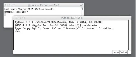
When you launch IDLE in a terminal window, you should see windows like the ones shown in Figure 1.1 (Mac OS version). Hereafter, the IDLE shell is simply called theshell.
Figure 1.1
If the version number displayed in the shell is not 3.3.4 or higher, you need to close the shell window and download and install the current version of Python, as described earlier.
The shell provides a“sandbox”where you can try out simple Python code fragments. To run a code fragment, you type it after the>>>symbol and press the Return or Enter key. The shell then responds by displaying a result and giving you another >>> prompt. Figure 1.2 shows the shell and its results after the user has entered several Python code fragments.
Figure 1.2
The shell after entering several code fragments.
© 2014 Python Software Foundation.
Some of the text is color-coded (blue, green, and red) in your shell window, although these colors do not appear in this monochrome book. The colors indicate the roles of var-ious code elements, to be described shortly.
To repeat the run of an earlier line of code, just place the cursor at the end of that line and press Return or Enter twice.
When you are ready to quit a session with the shell, you just select the shell window’s close box or close the associated terminal window. However, keep a shell handy when reading this book, so you can try out each new idea as you encounter it.
Obtaining Python Help
There are two good ways to get help when writing Python code:
1. Browse the Python documentation.
2. Run Python’shelpfunction in the shell.
Python’s helpfunction is especially useful for getting quick help on basic code elements, such as functions. For example, the use of Python’sabs function in Figure 1.2 might seem obvious to you, but if you’re not sure, you can learn more by enteringhelp(abs), as shown in Figure 1.3.
Figure 1.3
Getting help in the shell.
© 2014 Python Software Foundation.
Working with Numbers
Almost all computer programs use numbers in some way or another. In this section, you explore arithmetic with two basic types of numbers in Python: integers and floating-point numbers. Along the way, the important concepts of variables, assignment, functions, and modules are introduced.
Using Arithmetic
As you know from mathematics, integers are the infinite sequence of whole numbers {..., –2, –1, 0, 1, 2, ...}. Although this sequence is infinite in mathematics, in a computer program the sequence is finite and thus has a largest positive integer and a largest negative integer. In Python, the sequence of integers is quite large; the upper and lower bounds of the sequence depend on the amount of computer memory available.
Real numbersare numbers with a decimal point, such as 3.14 and 7.50. The digits to the right of the decimal point, called thefractional part, represent theprecisionof a real num-ber. In mathematics, real numbers have infinite precision. The set of real numbers is also infinite. However, in a computer program, real numbers have an upper bound, a lower bound, and a finite precision (typically 16 digits). In Python and most other programming languages, real numbers are calledfloating-point numbers.
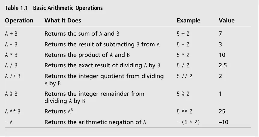
(without the buttons). Python’s basic arithmetic operations are listed in Table 1.1. In this table, the symbols A and B can be either numbers or expressions containing numbers and operators.
Table 1.1 Basic Arithmetic Operations
Operation What It Does Example Value
A + B Returns the sum ofAandB 5 + 2 7
A–B Returns the result of subtractingBfromA 5–2 3
A * B Returns the product ofAandB 5 * 2 10
A / B Returns the exact result of dividingAbyB 5 / 2 2.5
A // B Returns the integer quotient from dividing
AbyB
5 // 2 2
A % B Returns the integer remainder from dividingAbyB
5 % 2 1
A ** B ReturnsAB 5 ** 2 25
–A Returns the arithmetic negation ofA –(5 * 2) –10
Note the following points about the arithmetic operations:
1. The /operator produces the exact result of division, as a floating-point number. 2. The //operator produces an integer quotient.
3. When two integers are used with the other operators, the result is an integer.
4. When at least one floating-point number is used with the other operators, the result is a floating-point number. Thus,5 * 2 is 10, whereas 5 * 2.3is 11.5.
As in mathematics, the arithmetic operators are governed byprecedence rules. If operators of the same precedence appear in consecutive positions, they are evaluated in left-to-right order. For example, the expression3 + 4–2 + 5is evaluated from left to right, producing 10.
When the operators do not have the same precedence,** is evaluated first, then multipli-cation (*,/,//, or%), and finally addition (+or–). For example, the expression4 + 3 * 2 ** 3 first evaluates2 ** 3, then3 * 8, and finally4 + 24, to produce 32.
You can use parentheses to override these rules. For example,(3 + 4) * 2 begins evaluation with the addition, whereas3 + 4 * 2begins evaluation with the multiplication. What are the results of evaluating these two expressions? Open a shell and check!
Negative numbers are represented with a minus sign. This sign is also used to negate more complex expressions, as in –(3 * 5). The precedence of the minus sign when used in this way is higher than that of any other arithmetic operator.
Table 1.2 shows the precedence of the arithmetic operators, where the operators of higher precedence are evaluated first.
Table 1.2 The Precedence of Arithmetic Operators
Operator Precedence
–(unary negation) 4
** 3
*,/,//,% 2
+,–(binary subtraction) 1
The exponentiation operator ** is also right associative. This means that consecutive ** operators are evaluated from right to left. Thus, the expression 2 ** 3 ** 2 produces 512, whereas(2 ** 3) ** 2produces 64.
Finally, a note on style: although Python ignores spaces within arithmetic expressions, the use of spaces around each operator can make your code easy for you and other people to read. For example, compare
34+67*2**6–3
to
34 + 67 * 2 ** 6–3
Working with Variables and Assignment
Suppose you are working on a program that computes and uses the volume of a sphere. You are given the sphere’s radius of 4.2 inches. You first compute its volume using the formula 4/3πr3, with 3.1416 as your estimate of π. Here is the Python expression you might write for that:
If the value of this expression is used just once in your program, you compute it just once and use it there. However, if it is used in several places in your program, you must write the same expression several times. That’s a waste of your time in writing code and a waste of the computer’s time in evaluating it. Is there a way to write the expression, compute its value just once, and then simply use this value many times thereafter?
Yes, there is, and that’s one reason why programs usevariables. A variable in Python is a name that stands for a value. A Python variable is given a value by using the assignment operator=, according to the following form:
variable = expression
where variable is any Python name (with a few exceptions to be discussed later) and expression is any Python expression (including the arithmetic expressions under discus-sion here). Thus, in our example, the variable volume could be given the volume of the sphere via the assignment
volume = 4 / 3 * 3.1416 * 4.2 ** 3
and then used many times in other code later on. Note that because the precedence of assignment is lower that that of the other operators, the expression to the right of the = operator is evaluated first, before the variable to the left receives the value.
Now, suppose you had to compute the volumes of several different spheres. You could type out the expressions 4 / 3 and 3.1416 every time you write the code to compute a new volume. But you could instead use other variables, such as FOUR_THIRDS and PI, to make these values easy to remember each time you repeat the formula. Figure 1.4 shows a session in the shell where these values are established and the volumes of two spheres, with radii 4.2 and 5.4, are computed.
Figure 1.4
Using variables in code fragments.
© 2014 Python Software Foundation.
Python variables are spelled using letters, digits, and the underscore (‘_’). The following rules apply to their use:
n A variable must begin with a letter or an underscore (‘_’) and contain at least one letter.
n Variables are case sensitive. Thus, the variablevolume is different from the variable Volume, although they may refer to the same value.
n Python programmers typically spell variables in lowercase letters but use capital
letters or underscores to emphasize embedded words, as in firstVolumeor first_volume.
n When the value of a variable will not change after its initial assignment, it’s considered a constant. PIis an example of a constant. Python programmers typically spell constants using all caps to indicate this.
n Before you can use a variable, you must assign it a value. An attempt to use a variable that has not been initialized in this way generates an error message, as shown in Figure 1.5.
Figure 1.5
Attempting to use a variable that has not been assigned a value.
© 2014 Python Software Foundation.
To summarize, there are three reasons to use variables in Python code:
1. They make code easy to read and understand.
2. They help to eliminate unnecessary computations.
Using Functions
As you have seen, the arithmetic and assignment operations consist of an operator and one or more operands. Python also provides many other basic operations, which are pack-aged asfunctions. A function is like an operator but is referred to by a name rather than an operator symbol. When a function is evaluated or called, its operands are supplied to it in the form of arguments. For example, the Python function abs expects a number as its single argument and computes and returns that number’s absolute value. Thus, the func-tion callabs(-34)returns 34.
When a Python function is called, Python first evaluates its arguments. The resulting values are then passed to the function, which uses them to compute and return its value. Although the written form of a function call is slightly different, the process is no different from evaluating an expression with operands and operators. The form of a function call is as follows:
functionName(argumentExpression-1, argumentExpression-2, ...)
Function calls are expressions, and their arguments are expressions. For example, the arithmetic expression
abs(length - width) + 2
produces a result, as long as the variableslengthand width refer to numbers.
Some Python functions allow for optional arguments as well as required arguments. For example, the Python function round expects one required argument: the number to be rounded. If that number is a floating-point number, the integer value nearest to it is returned. However,roundcan also be called with a second argument: an integer indicating the number of places of precision to use in the result. Thus, round(3.1416) returns 3, whereasround(3.1416, 3)returns 3.142.
Generally, the number of arguments used with a function must match the number of its required arguments, unless it allows optional arguments. For functions provided by Python, the types of the arguments (such as numbers) used must also match the types of the arguments expected at each position in the sequence of arguments.
Using the math Module
Python’s functions either are already available to call in the shell or must be imported from modules before use. A Python module is just a library of functions and other resources. There are many such modules, as you can see by browsing the modules index
in the Python documentation. One of these is the math module, which contains useful functions for operations on numbers.
There are several ways to import a function from a module to make it available for use. The most common way is to use the form
importmoduleName
wheremoduleName is the name of the module. When you have done this, you can call any function in the module by using the form
moduleName.functionName(sequenceOfArguments)
For example, suppose you want to compute the square root of 2. The following shell session shows how to do this:
>>> import math >>> math.sqrt(2) 1.4142135623730951
Alternatively, if you prefer not to use the module name as a prefix in a function call, you can explicitly import the desired function, as follows:
>>> from math import sqrt >>> sqrt(2)
1.4142135623730951
To view all the functions available in themathmodule, you run dir(math)after importing math, as follows:
>>> import math >>> dir(math)
[’__doc__’,’__file__’,’__loader__’,’__name__’,’__package__’,’acos’,’acosh’,’asin’,
’asinh’,’atan’,’atan2’,’atanh’,’ceil’,’copysign’,’cos’,’cosh’,’degrees’,’e’,
’erf’,’erfc’,’exp’,’expm1’,’fabs’,’factorial’,’floor’,’fmod’,’frexp’,’fsum’,
’gamma’,’hypot’,’isfinite’,’isinf’,’isnan’,’ldexp’,’lgamma’,’log’,’log10’,
’log1p’,’log2’,’modf’,’pi’,’pow’,’radians’,’sin’,’sinh’,’sqrt’,’tan’,’tanh’,
’trunc’]
Now you can use this value to compute a more precise volume of a sphere than you did earlier, using the following statement:
volume = FOUR_THIRDS * math.pi * radius ** 3
Another way to access the items in a module is to import all of them explicitly. To do this with themathmodule, you run
from math import *
To access help on any module function, run the helpfunction on the function’s name. If you’ve imported just the module, you use the form
help(moduleName.functionName)
Otherwise, you use the form
help(functionname)
To get help on an entire module after importing it, runhelpon the module’s name. You might be thinking,“Hey, why doesn’t themathmodule include a function to compute the volume of a sphere? Then I could just give that function the radius and let it do all the work.” That would be a nice function to have, but the folks at python.org could not pro-vide a function for every occasion. Later in this book, you learn how to create your own functions and modules to add to Python’s built-in capabilities.
Detecting Errors
Figure 1.6 shows a shell session with several errors in Python code.
Figure 1.6
Examples of errors in Python code.
© 2014 Python Software Foundation.
There are three types of errors that can occur in your code:
n Syntax errors—These errors occur when your code is not well formed, according to the syntax or grammar rules of Python. For example, the expressionabs(-34)is syntactically correct, but the expression abs(-34))is not. (It contains an extra right paren.)
n Semantic errors—These errors occur when a syntactically correct expression is evaluated, but Python cannot carry out the evaluation. For example, Python cannot divide a number by zero, cannot compute the square root of a negative number, and cannot use a variable that has not yet been given a value, even though you can enter each such expression in the shell without a syntax error.
n Logic errors—Also called design errors, these errors occur when Python successfully evaluates an expression, but the expression returns an incorrect result. For example, the expression math.pi * 34 ** 2does return a value, but if you expect this value to be the volume of a sphere of radius 34, your code contains a logic or design error.
Python detects syntax and semantic errors automatically and displays error messages. However, you must detect logic or design errors yourself by testing and inspecting the results of your code. In advanced software development settings, programmers can use software tools to automate some of this testing as well.
In general, you should regard error messages with a friendly eye and learn to understand what they mean. As you become a competent programmer, you will have few syntax and semantic errors in your code, so you can turn your attention to eliminating any logic errors.
Working with Strings
Text processing is almost as prevalent in computing as numerical processing. Instant mes-saging, texting, and word processing would be impossible without it. In this section, you explore working with strings, which form the basis of text processing.
String Literals
ses-Figure 1.7
Examples of strings in Python.
© 2014 Python Software Foundation.
Note that you can use pairs of single quotes, pairs of double quotes, or pairs of triple-single or triple-double quotes. Strings enclosed in triple-single quotes or double quotes cannot extend to the next line of code. Strings enclosed in triple quotes can extend to multiple lines of code, but the line breaks are included as characters within these strings.
Note also that, like numbers, strings evaluate to themselves, but the results are displayed in single quotes.
If you want to embed quotes within a string, you can place the escape character\ imme-diately before the embedded quote. The escape character is also used to embed special characters, such as the Tab and Return characters, within a string. Table 1.3 lists some escaped characters and their meanings.
Table 1.3 Some Escaped Characters
Character Meaning
\n Newline (Return or Enter)
\t Horizontal Tab
\\ \
\’ ‘
\” “
Strangely enough, the empty string, represented as“”, is still a string, even though it con-tains no characters.
The len, str, int, and float Functions
A string’s length is the number of characters it contains. The len function allows you to look up the length of its string argument, as shown in the next shell session:
>>> len("") 0
>>> len("Here are four words.") 20
Note that the empty string contains no characters, whereas the space counts as a character.
Thestr function converts its argument to a string representation. In the case of numbers, str has the effect of wrapping the number in a set of quote marks. The str function is often used to build text from other types of data values, such as numbers.
Theintand floatfunctions are used to build numbers from strings. Note that a string of digits does not look very different from a number that contains the same sequence of digits, but they are very different species of data from Python’s point of view. The follow-ing shell session illustrates this difference and shows some uses of the int and float functions:
>>> 34 + 22 56
>>> "34" + "22"
’3422’
>>> "34" + 22
Traceback (most recent call last):
File "<pyshell#10>", line 1, in <module> "34" + 22
TypeError: Can’t convert’int’object to str implicitly >>> str(22)
’22’
>>> "34" + str(22)
’3422’
>>> int("34") 34
>>> int("34") + 22 56
>>> int(3.6) 3