PRODUCTION VARIABLE ANALYSIS
FOR ADEQUATE AVAILABILITY OF DOMESTIC SOYBEAN
PRODUCTION
Nelly Budiharti1, Sanny Anjarsari2, Emma Adriantantri3
1,2,3 Lecturer of Industrial Engineering, National Institute of Technology, Malang , Indonesia
Email : [email protected]
ABSTRACT: Soybean plants are easily found in most provinces in Indonesia. However, the production capacity in each province is unbalanced. Therefore, it is necessary to analyze the factors that influence the soybean production capacity. This research is conducted using surveys, interviews and questionnaire. The sample is taken from the Gapoktan (Group Chairman Farming Association), Kapoktan (Chairman of the Farm) and individual soybean farmers in Jember and Banyuwangi villages, East Java, Indonesia. The soybean production variable has eight indicators and the soybean stock variable has two indicators. Data analysis is done by calculating the average value (mean). The results show that the average value (mean) was 4.44 using 5 point Likerts Scale. Therefore the data is valid and reliable. The relationship between the variable and the indicator has a strong correlation with an average of 0.96 and it follows the quadratic model. The hypothesis results show that there are influences and strong relationship between the production variable and the stock variable. The strong dominant indicators are the use of abandoned land and utilization of forestry land or plantation.
Keywords: Availability, Domestic Soybean Production, Measurement Model, Production analysis
1. Introduction
Soybean demand in Indonesia is very high but the production capacity couldn’t meet the demand (Nurhayati, Nuryadi, Basuki, and lndawansani, 2010; Supadi. 2008; Suyamto, Widiarta, 2010). Most provinces in Indonesia cultivate soybean, but the production capacity of each province is unbalanced. According to (BPS, 2015), East Java province produces the highest soybean production, i.e. 35.8% from the total production in Indonesia. Central Java, West Nusa Tenggara, and West Java produce 13.5%, 13.0%, and 10.3% respectively. There is a big different in the production capacity between the first rank and the second, third, fourth ranks. This situation leads us to examine the factors that influence the production capacity.
2. Methodology
This research is conducted by means of surveys, interviews and questionnaire utilizing Likert scale of 5. Samples were taken from the Gapoktan (Joint Chairman of the Farm), Group Farming (Kapoktan) and Individual farmers for domestic soybean production. The study is conducted in Jember and Banyuwangi village as primary data, while secondary data is obtained from previous research and related documents, such as from the Central Bureau of Statistics and the Ministry of Agriculture at the district, province and national levels as well as the respective relevant agencies and their websites.
Mburugu, 2013; Nurhayati, Nuryadi, Basuki, and lndawansani, 2010; Setiawan, 2009; Sinar Tani. 2013; Supadi, 2008; Suyamto, Widiarta, 2010). The eight indicators for production variable are: 1) Monoculture planting; 2) Intercropping planting; 3) Year-round planting; 4) Utilization of abandoned land; 5) Land or plantation utilization or other uses, 6) Technology used; 7) Plant disruption organism control; and 8) Climate change impact control. The two indicators for stock variable are: 1) Planting area; 2) Land function transfer.
Data are analyzed by calculating average value (mean), reliability validation, reliability and pattern model, and hypothesis test using SPSS 17 software for Windows. The validity of model and hypothesis were tested using Smart PLS Version 2.0 M3 software.
3. Results and Discussions
3.1 Descriptive Analysis
The results for of the frequencies distribution and the mean values for all respondents are given in Table 1 for production variable and Table 2 for stock variable, where scale of 1 is strongly disagree; 2 is disagree; 3 is doubtful; 4 is agree; and 5 is strongly agree.
Table 1 Description Indicator: Production Variable
Table 2 Description Indicator: Stock Variable
Indicator Y
Responses of respondents
Mean
1 2 3 4 5
f % f % f % f % f %
Y1 0 0 1 2.381 1 2.381 14 33.33 26 61.9 4.55
Y2 0 0 0 0 4 9.524 12 28.57 25 59.52 4.4
Mean Average 4.475
From Table 1 it is obtained that the mean average of respondents’ answers is 4.44. It means that most of respondents agree with eight indicators of production variable. From Table 2 it is
Indicator X
Responses of respondents
Mean
1 2 3 4 5
f % f % f % f % f %
X1 0 0 0 0 0 0 17 40.48 25 59.52 4.6
X2 0 0 0 0 0 0 23 54.76 19 45.24 4.45
X3 0 0 0 0 0 0 25 59.52 17 40.48 4.4
X4 0 0 0 0 7 16.67 15 35.71 20 47.62 4.31
X5 0 0 0 0 7 16.67 14 33.33 21 50 4.33
X6 0 0 0 0 4 9.524 7 16.67 31 73.81 4.64
X7 0 0 0 0 6 14.29 15 35.71 21 50 4.36
X8 0 0 0 0 7 16.67 15 35.71 20 47.62 4.31
obtained that the mean average of respondents’ answers is 4.475. It means that most of respondents agree with two indicators of stock variable.
3.2 Validity and Reliability
Statements given to the respondents should be tested. It is important therefore to verify the reliability and validity of the instruments, whether they are correct or appropriate to the investigated issues and whether the answers are consistent. The results are given in Table 3 and Table 4.
Table 3 Result of Validity and Reliability Test for X Variable
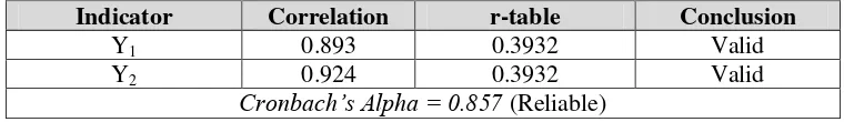
Table 4 Result of Validity and Reliability Test for Y Variable
Indicator Correlation r-table Conclusion
Y1 0.893 0.3932 Valid
Y2 0.924 0.3932 Valid
Cronbach’s Alpha = 0.857 (Reliable)
Table 3 shows that the correlation of all indicators (r) are greater than 0.3932. Thus all indicators of X variable are valid. Further, since the value of Cronbach’s Alpha is greater than 0.60 (i.e. 0.969), the instrument is reliable.
Table 4 shows that the correlation of all indicators (r) are greater than 0.3932. Thus all indicators of Y variable are valid. Further, since the value of Cronbach’s Alpha is greater than 0.60 (i.e. 0.857), the instrument is reliable.
3.3 Linearity Assumption Test
To determine the relationship between variables and indicators in accordance to the model, the curve estimation (Kutner, Nachtsheim, and Neter, 2004) is performed as given in Table 5. From the table, it is shown that the highest R2 is the quadratic model. While the linear model has the lower value of R2. Table 6 shows the linearity assumption of X and Y variables. From the table, it is shown that the relationship between the variables follows the linearity assumption, since the value of F deviation from linearity lies in the range of “not significant” (F=0.343; p=0.847; p>0.05).
3.4 Model Measurement Test
Model measurement test is performed to find the contribution of each indicator to its variable. All indicators in X variable are reflective, thus the outer loading analysis is used. While all
Indicator Correlation r-table Conclusion
X1 0.862 0.3932 Valid
X2 0.875 0.3932 Valid
X3 0.812 0.3932 Valid
X4 0.985 0.3932 Valid
X5 0.981 0.3932 Valid
X6 0.804 0.3932 Valid
X7 0.973 0.3932 Valid
X8 0.985 0.3932 Valid
indicators in Y variable are formative, thus outer weight analysis is used. The results are given in Table 7 and Table 8.
Table 5 Model Summary and Parameter Estimation
Dependent Variable: Y
Equation
Model Summary Parameter Estimates
R2 F df1 df2 Sig. Constant b1 b2 b3
Linear .862 249.608 1 40 .000 2.533 .184
Logarithmic .830 195.266 1 40 .000 -12.741 6.125
Inverse .792 152.000 1 40 .000 14.803 199.945
Quadratic .938 297.359 2 39 .000 19.790 -.841 .015
Cubic .937 291.979 2 39 .000 14.306 -.343 .000 .000
Compound .861 247.517 1 40 .000 4.354 1.021
Power .830 195.264 1 40 .000 .792 .683
S .793 152.875 1 40 .000 2.840 -22.317
Growth .861 247.517 1 40 .000 1.471 .021
Exponential .861 247.517 1 40 .000 4.354 .021
Logistic .861 247.517 1 40 .000 .230 .980
Table 6 Anova Table
Sum of
Squares df
Mean
Square F Sig.
Y * X
Between Groups (Combined) 41.794 5 8.359 .350 .879
Linearity 8.962 1 8.962 .375 .544
Deviation
from Linearity 32.832 4 8.208 .343 .847
Within Groups 860.682 36 23.908
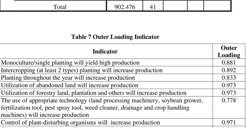
Total 902.476 41
Table 7 Outer Loading Indicator
Indicator Outer
Loading
Monoculture/single planting will yield high production 0.881
Intercropping (at least 2 types) planting will increase production 0.892
Planting throughout the year will increase production 0.833
Utilization of abandoned land will increase production 0.973
Utilization of forestry land, plantation and others will increase production 0.973 The use of appropriate technology (land processing machinery, soybean grower,
fertilization tool, pest spray tool, weed cleaner, drainage and crop handling machines) will increase production
0.778
Control of plant-disturbing organisms will increase production 0.971
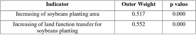
Table 8 Outer Weight Indicator
Table 7 shows that the highest contribution to the increasing of production is achieved by the indicators that have the highest outer loading, i.e. 0.973. The positive value of outer loading indicates the positive contribution of the indicator to its variable.
Table 8 shows that both indicators contribute to the increasing of stock variable. The contributions of indicators are very significant since the p value is lower than 0.05,
3.5 Hypothesis Test
The hypothesis test X variable to Y variable is performed to find the relationship and impact of the production variable to the stock variable. The important parameters should be considered are Chi-square and Asymp Sig. The decision rule is as follows:
a. If calculated X2 > X2 of the table, then H0 is accepted: There is a relationship between
production variable and stock variable.
If calculated X2 < X2 of the table, then H1 is accepted: There is no relationship between
production variable and stock variable.
b. If probability > 0.05, then H0 is accepted: There is a relationship between production
variable and stock variable.
If probability < 0.05, then H1 is accepted: There is no relationship between production
variable and stock variable.
The results from SPSS software is as follows:
- The calculated X2 = 14.951
- The X2 of table = 14.68366
- Probability of significance = 0.092
- α = 0.10
According to the results, the conclusion is
1. Since (calculated X2 = 14.951) > (X2 of table = 14.68366), then H0 is accepted: There is
a relationship between production variable and stock variable.
2. Since (probability of significance = 0.092) > 0.092, then H0 is accepted: There is a
relationship between production variable and stock variable.
4. Conclusion
In the research, the survey to find relationship between the production variable and stock variable of soybeans plant in Indonesia is conducted. The respondents agree that there is a relationship between the production variable (with eight indicators) and the stock variable (with two indicators). The relationship follows the quadratic model. The dominant indicators are utilization of abandoned land and utilization of forestry land, plantation and others. The correlation between each variable and its indicator is very high.
Indicator Outer Weight p value
Increasing of soybeans planting area 0.517 0.000
Increasing of land function transfer for soybeans planting
References
BPS. 2015. https://www.bps.go.id/linkTableDinamis/view/id/871
Directorate General of Food Plants. 2010. Road Map of Increased Soybean Production Years 2010 – 2014. Ministry of Agriculture, Jakarta.
Irwan. 2013. Determinants and Decisions Factor for Farmers in the Selection of Varieties of Soybean Seeds in Pindi Regency. Agrisep, Vol. 14, No. 1.
Ishaq, M.N., Ehirim, B.O. 2014. Improving Soybean Productivity Using Biotechnology Approach in Nigeria. World Journal of Agricultural Sciences, Vol. 2, No. 2, pp. 13-18. Khanh, T.D., Anh, T.Q., Buu, B.C., and Xuan, T.D. 2013. Applying Molecular Breeding to
Improve Soybean Rust Resistance in Vietnamese Elite Soybean. American Journal of Plant Sciences, Vol. 4, pp. 1-6.
Kutner, M. H., Nachtsheim, C.J. and Neter, J. 2004. Applied Linear Regression Models. 4th ed, McGraw-Hill/Irwin, Boston
Mahasi, J.M., Mukalama, J., Mursoy, R.C., Mbehero, P., Vanluwe, A.B. 2011. A Sustainable Approach To Increased Soybean Production In Western Kenya. African Crop Science Conference Proceedings, Vol. 10, pp. 115 – 120.
Njeru, E.M., Maingi, J.M, Cheruiyot, R., and Mburugu, G.N. 2013. Managing Soybean for Enhanced Food Production and Soil Bio-Fertility in Smallholder Systems through Maximized Fertilizer Use Efficiency. International Journal of Agriculture and Forestry, Vol. 3, No. 5, pp. 191-197.
Nurhayati, Nuryadi, Basuki, and lndawansani. 2010. Analysis of Climate Characteristics For Optimizing Soybean Production in Lampung Province. Final Report of PKPP Ristek, 2010 Meteorology and Geophysics Research and Development Center. (In Indonesian)
Setiawan, E. 2009. Local Wisdom of Cropping Pattern in East Java, Jurnal Agrovigor,Vol. 2, No. 2. (In Indonesian)
Sinar Tani. 2013. Development of Soybean in Forest Area as a Source Seed. Agroinivasi, Edition 15, No. 3470, August 2, 2012, XLII, Research and Development Body of Agriculture.
Supadi. 2008. To Encourage the Participation of Farmers for Increasing the Soybean Production Towards the Self-sufficiency. Journal of Research and Development of Agriculture, Vol. 27, No. 3. (In Indonesian)