Applications
Patrik Alfredsson  Olof WååkSystecon AB, Box 5205, SE-102 45 Stockholm, Sweden
This paper shows that
a) the constant demand rate assumed by all multi-item, multi-echelon, multi-indenture spares optimization models is a very good approxima-tion also if components are assumed to have non-constant failure rate distributions
b) the potential error in assuming constant demand rates is negligible compared to other uncertainties or errors generic to all practical appli-cations
c) renewal processes are, except for Poisson processes, directly unsuit-able for practical problem solving related to logistics support analysis and spares requirements; the possible exception is one-component-per-item (single-indenture), single-system, single-site problems
Furthermore, we motivate why simulation, although an excellent tool for analysis of given situations or decisions, is seldom applicable for optimi-zation.
(Inventory Control; Spare Parts; Failure Rate; Demand Processes)
1.
Introduction
Much of the research within the field of reliability concerns non-constant failure rates, that is, the distribution for the time between failures is assumed not to be an
exponen-tial distribution. Seemingly in contrast, most practical applications within the field of logistic support assume constant failure rates, or rather constant demand rates. This
paper focuses on applications related to spares optimization. All item, multi-echelon, multi-indenture spares optimization models assume constant demand rates (see, for example, [She68], [Muc68], [Gra85], [She86] and [Sys98]). Are they wrong in doing so? The purpose of this paper is to clarify the picture, and in particular point out the difference between demand processes for spares and component failure proc-esses. Hopefully this will remedy some misconceptions about spares optimization models like OPUS10 [Sys98].
that inventory control of spare part stocks is governed by spares demand and not by component failures (although, of course, most component failures will indirectly
re-sult in spares demand). Therefore, we put emphasis on describing the relationships and differences between component failure processes and demand processes for spares. The primary objective is to show and motivate why it is reasonable to assume constant demand rates without assuming constant component failure rates.
Theoretically we shall rely on classical limit results presented by Drenick and Khintchine. In most instances, the demand process for spares at a given site is the su-perposition (or pooled output) of a number of failure and/or demand processes. It is shown by Drenick that, under extremely mild conditions, the superposition of inde-pendent stationary failure (demand) processes will in the limit (as the number of proc-esses increases) tend to a Poisson process. A similar but more general result is proved by Khintchine. We illustrate the implications of these results by simulation in sec-tion 6.
Furthermore, Poisson processes possess certain properties that make them the only practical choice when modeling complex multi-echelon, multi-indenture support system. For example, the class of Poisson processes is closed under superposition, and the probabilistic split of a Poisson process yields independent Poisson processes. The expression closedness under superposition is perhaps technical but extremely
con-venient and we will frequently use it. It simply means that if we superpose (that is, merge or “add”) two or more Poisson processes the result is a Poisson process. When superposing a number of arbitrary stationary processes, it is difficult to characterize the ‘true’ pooled process. As a result, non-Poisson approaches are confined to single-system, one-component-per-item situations that are infrequent and normally of little practical interest when determining the optimum sparing strategy for a real-world technical system. We believe that non-Poisson approaches could perhaps be justified for reliability and maintenance analyses that tend to be on the component level, but not for logistic support analyses and spares optimization.
2.
Preliminaries
Central to the discussion in this paper are a few objects that need to be defined. On the macro level we have two fundamental objects known as the technical system and the support system. The technical system will act as a generator of maintenance tasks that
the support system shall perform. Our main focus is on finding optimum sparing poli-cies, and hence we focus on maintenance tasks leading to spares demand. Such tasks can be of a corrective as well as a preventive or scheduled nature. Note that in many cases the technical system consists of a number of individual systems. Think, for ex-ample, of a fleet of aircraft.
On the micro level we have so called components. These are the smallest parts
of the technical system that can generate a preventive or corrective maintenance task. In other words, a component is a leaf of the system break-down tree. Since the level of system break down can be somewhat arbitrarily chosen, the definition of a component is somewhat ambiguous. From a practical point of view, however, this ambiguity causes no problem why we do not elaborate on this issue. Typical components could be resistors, transistors, nuts, bolts, etc.
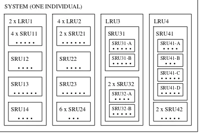
subitems form items, and items form individual systems (see Figure 1). These hierar-chical levels are referred to as the indenture levels of the system. Items that are re-placed directly in the system are called first-indenture or primary items. Thus, to
re-pair or maintain the technical system, spare parts of primary items are demanded. Furthermore, second-indenture or secondary items are replaced to repair or maintain a
primary item. Continuing in this fashion we eventually reach the components that are normally but not necessarily discarded. The terms LRU (Line Replaceable Unit) for primary units and SRU (Shop Replaceable Unit) for secondary units and beyond are often used.
The failure characteristics of a component can be described in several ways. One way is to use the continuous random variable T, the time to failure of the component.
(One normally assumes identical failure characteristics for all individuals of a given component type.) In turn, the properties of the random variable T can be described in
several equivalent ways, that is, by its • distribution function, F t( ) =Ρ
[
T ≤t]
,• (instantaneous) failure rate or hazard function, z t( )
The instantaneous failure rate is defined as
[
]
Thus, it reflects the components tendency to fail at time t given that it has survived up
Finally, note that from the above relationships it follows that a component has con-stant incon-stantaneous failure rate if and only if the distribution for time to failure is an exponential distribution.
The name (instantaneous) failure rate for z t( ) is commonly used (and therefore
accepted) although rather unfortunate and a source of confusion. Normally, by a rate we mean the number of occurrences per time unit which has a straightforward physi-cal meaning. The function z t( ) , however, is defined as a conditional probability per
time unit, which is clearly a more theoretical quantity. Hence, a constant failure rate could mean that the number of occurrences per time unit does not vary over time, but instead normally means that the conditional probability of failure per time unit is con-stant.
The true distribution function of T is never known and we consequently have to
estimate it. Following the so called parametric approach we approximate the true dis-tribution with a disdis-tribution taken from a class of disdis-tribution functions described by a few (normally one or two) parameters. The estimation then amounts to choosing pa-rameter values so as to obtain the best possible fit. There are different ways to define the best fit, two of which are maximum likelihood and minimum least squares.
A class of distribution functions that is often used for component failures is the class of Weibull distributions. The distribution function for a Weibull-distributed ran-dom variable is given as
Furthermore, the failure rate function is given as
z t( )=βλ λ( )t β−1. (2.7)
The form of the failure rate function in (2.7) is a major reason for the popularity of the Weibull distribution in relation to component failures. By choosing 0< <β 1 the failure rate function is decreasing. For β =1 it is constant, and for β >1 it is in-creasing.
3.
Need for spares
When analyzing spares requirements the first thing we have to realize is that
The need for spares is determined by spares demand
Although this statement might look superfluous it is so fundamental that we like to emphasize it. So if we want to determine the amount of spares of LRU1 at site A we need to describe the demand process of LRU1 at site A. (Of course we also need to characterize the resupply process but this is not the focus of this paper.)
The demand process for a given item at a given site is formed by and dependent upon on several factors, some of which the more important are:
• failure generation in the components of the item
• degree of no fault found, that is, incorrectly reported failures • frequency of preventive maintenance by item replacement
• the number of individual systems that request spare items from the site in question • the number of items of the given type per individual system
• system utilization
In turn, the failure generation or failure processes of the components of the item depend upon
• intrinsic failure properties of the components • preventive maintenance actions
• corrective maintenance actions • equipment handling
• system utilization, for example, in terms of component stress and load over time Obviously, it is in general incorrect to equate the demand process for a spare item by the intrinsic failure process of one component mounted in one system. Note, however, that when claiming that a constant demand rate necessitates a constant fail-ure rate this is in reality what we do. In most cases, the demand process for a given item type at a given site is the result (in essence the superposition) of a number of component failure processes. Firstly, there is often a number of systems that request spare items from the same site. Secondly, there could be several items of the given type mounted in each system. Thirdly, there are often a large number of components within each item.
support organization is supplied a minimum of around 20 systems. This means that demand process for each radar LRU at each site is the superposition of at least around 38,000 component failure processes. Clearly, it is cumbersome not to say impossible task to derive the exact demand processes based on the component failure processes. Furthermore, it is unrealistic to assume that we know the component failure processes. At best, we can look up intrinsic failure properties of components in a clinical envi-ronment, under certain operating conditions. As indicated above, the true failure proc-ess depends many other factors, for example, preventive maintenance. It is generally accepted that preventive maintenance affects the failure properties of components, al-though it is debated whether in a positive or negative direction.
The sizable multiplicity, although seemingly problematic, is in fact extremely beneficial when we seek to characterize the demand processes for different kinds of
spares. It motivates and validates the application of classical limit theorems concern-ing the superposition of stationary (renewal) processes.
Theorem 1 (Drenick). Given N components, indexed by i =1, ,Κ N , whose failure processes are independent equilibrium (stationary) renewal processes, let F ti( ) be the distribution for time between failures of component i. Furthermore, λi denotes the
expected number of renewals per time unit, that is, 1 λi is the expected time between failures of component i. Let GN( )t be the distribution for time between failures across all components, that is, the time between events in the pooled process. If
(i) lim sup
Consequently, Drenick’s theorem [Dre60] states that, under the above assump-tions, the pooled output will approach a Poisson process as the number of processes increases. Condition (i) is technical and non-restrictive. Condition (ii) is satisfied by all failure distributions commonly used, for example, the Weibull distribution (see the previous section). Khintchine [Khi60] proves a similar theorem to Drenick’s that holds for independent stationary processes, not necessarily renewal processes.
In connection to spares demand we draw the following conclusion:
When the demand process for an item at a site is the result of several com-ponent failure processes (which it normally is), the demand process tends to be (or be well approximated by) a Poisson process, that is, the demand rate is (approximately) constant. The individual components can have basically arbitrary failure properties.
4.
Methods and models for spares optimization
As we see it, there are only a few quantitative methods available when determining spares requirements. We identify them as analytical methods based on constant de-mand rates, analytical methods based on renewal theory, and simulation methods. As have become clear, we favor analytical methods based on constant demand rates. Let us begin by motivating why simulation methods are generally impractical when per-forming spares optimization (or, in fact, any kind of optimization).
Event-driven simulation is an extremely general idea that can be applied to
analyze basically any stochastic system or process. In terms of optimization, however,
it is seldom, not to say never, applicable. The reason for this is time, or more pre-cisely, the relatively extensive time required for a single function evaluation. Any op-timization algorithm evaluates the objective function (and/or its derivatives) numerous times in order to establish the optimal solution. If each function evaluation takes time, the optimization algorithm soon becomes impractical. To illustrate, let us assume that each function evaluation by simulation takes one second, and that to find the optimal solution requires ten billion (1010) function evaluations. Then it would take more than
300 years to find the optimal solution. The reader that thinks that 1010 is a large
num-ber should bear in mind that this is the numnum-ber of solutions for 10 items for which the stock level at one site can vary between 0 and 9. In the spares optimization setting, which is combinatorial in nature, 1010 is not a large number!
In the analytical world, function evaluation is generally much faster and optimi-zation feasible. The classes of analytical models we identify and like to compare are those based on Poisson demand (constant demand rate), and those based on general renewal processes. The reason is that the component failure processes are naturally described by renewal processes.
The theory of renewal processes is well-developed and mature and several books have been written on the subject (see, for example, [Cox62]). An (ordinary) newal process is characterized by one entity, the distribution for the time between re-newals, denoted F t( ) . If F t( )= −1 e−λt then the renewal process is a Poisson process
with rate λ. Hence, the renewal process is a generalization of the Poisson process. Note, however, that several properties of the Poisson process are not inherited by arbitrary renewal processes. Most importantly, the superposition of two independ-ent renewal processes is not a renewal process unless both processes are Poisson processes. When modeling a multi-echelon, multi-indenture support system, demand
processes are ultimately formed by superposition of other processes (see section 2). The lack of closedness under superposition makes the class of renewal processes an implausible class to work with. Similarly, the probabilistic split of a renewal process does not yield independent renewal processes. The probabilistic split of a (point) pro-cess into M processes is constructed in the following way. Given
{
N t t( ): >0 , the}
original process, each event leads to an event in one and only one of the processes
{
N t ti( ): >0 , 1}
≤ ≤i M. The probabilities are pi respectively, and they are inde-pendent of previous events.compo-nent failure processes as renewal processes, the spare item demand process is not a renewal process. Of course, we can approximate it to be a renewal process, but it is still not clear which. As argued in section 3 and seen in section 6, a good approxima-tion is to assume it to be a Poisson process. In effect, renewal processes do not lend themselves to superposition, and therefore models based on renewal theory have ited applicability in terms of spares optimization. As we see it, such models are lim-ited to single process (that is, single-system, one-component-per-item, single-item) situations that are rare when determining the optimum sparing strategy for a real-world technical system.
5.
Some comments on uncertainty
Applied mathematicians can build models based on whatever mathematical theory suitable for their purpose. The purpose is inevitably to describe the real world in terms of a set of mathematical relations, a mathematical model. From a more theoretical mathematician’s point of view, predominant design criteria are often the exactness and/or the generality of the model. By exactness we mean how well the model agrees with the reality. There is always a degree of uncertainty associated with the results, or with the description of reality produced by the model. We refer to errors related to this model uncertainty as model errors. Model errors or uncertainty reflect how well a
per-fectly tuned model would mimic a reality known to 100 percent.
Many (not to say most) mathematical models are parametric. This means that an instance of the real world is fed into the model in the form of a number of parameters. Thus, these parameters need to be estimated, and this is normally done by judgment, observations and measurements of real-world systems. Hence, there is uncertainty re-garding the correct values of the model parameters, and we refer to this uncertainty as parameter uncertainty. Related errors are called parameter errors. In reality, we never
know exactly the real world and thus we cannot perfectly tune our model.
A more theoretical mathematician will often ignore or neglect parameter uncer-tainty and focus on model unceruncer-tainty. For him there is no cost associated with zero parameter error - it is just an assumption - and he can concentrate his efforts on the accuracy of the model.
The world of a more applied mathematician (an operations analyst or a real-world problem solver) is however more complex, and to him zero parameter error at no cost is a fantasy. He must weigh errors, model as well as parameter, against the cost of decreasing them.
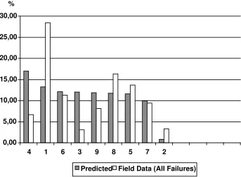
The above example illustrates the difficulty to correctly estimate mean demand at the earlier stages of the system life cycle. The predictions were made by a major, capable electronics company using state-of-the-art methods. It simply (and unfortu-nately) reflects the status of failure rate predictions. If we assume constant demand rates, these are the parameters we must feed to specify spares demand, and hence de-termine spares requirements.
When building a model based on renewal theory and non-constant rates, the pa-rameters we need to estimate increases drastically. Apart from the mean we must also estimate the spread (in terms of variance, or some other equivalent second-order quantity). In effect, we should also specify the distributions for times between renew-als of all processes, although to assume Weibull distributions seems to be in vogue. The difficulty of estimating the necessary parameters is noted and expressed by Crocker [Cro96]: “Even in retrospect, it is very rare that there will be sufficient fail-ures of a given mode on a given design (modification standard) of component to be able to determine with high confidence the “true” values of the parameters”. That is,
the parameter uncertainty is high when there is little field data available, and as he also notes, there is in general little (or no) field data available at the stages when spares analysis (or optimization) is to be performed.
So far we have primarily discussed uncertainty associated with spares demand processes. Of course, there is also uncertainty related to many other aspects of the support system and its operation, for example, the resupply processes (shipment and repair processes). The support system operates in a changing environment where new restrictions and requirements are imposed (see [Isd99]). Furthermore, the operations of the technical systems is uncertain, both in terms of mean utilization over time and operational profiles.
The point we like to make is that it is questionable (in fact, in many cases incor-rect) to spend money and effort on trying to reduce the model error by going from a
0,00 5,00 10,00 15,00 20,00 25,00 30,00
4 1 6 3 9 8 5 7 2
Predicted Field Data (All Failures) %
Poisson process to a more accurate demand process description. The model er-ror/uncertainty resulting from the Poisson approximation is small in relation to other sources of uncertainty. The “more accurate” model requires more input data (that is seldom available or costly to achieve) and is less applicable to real-world situations (for example, due to the lack of closedness under superposition).
6.
Simulation study of Drenick’s theorem
Many of our arguments and a lot of our reasoning in this paper is founded on Drenick’s (or Khintchine’s) theorem. Let us therefore more closely investigate Drenick’s theorem using simulation. We study how a spare stock behaves when the demand process is a superposition of a number of renewal processes. The two primary measures of effectiveness we look at are the expected number of backorders (NBO) and the risk of shortage (ROS). They are two fundamental measures often used for determining optimal sparing strategies.
In the first case we analyze, there are 100 (stochastically identical) processes su-perposed to form the spares demand process. Each event in a subprocess leads to spares demand, and if there is no spare available the individual process is halted until a spare is available. Apart from this, continuous operation (failure generation) is as-sumed for each process. The spares demand rate, with no process halted, is in total 0.01 demands per hour. For sake of simplicity, we assume a constant spare resupply time of 240 hours. Thus, with unlimited spares, there are on the average 2.4 units in resupply. The NBO and ROS values for stock levels (S) between 0 and 6 are analyzed
assuming the times between failures to be • exponential (exp), with mean 10,000 hours
• Weibull (W(2)), with shape parameterβ =2 and mean 10,000 hours • Weibull (W(4)), with shape parameterβ =4 and mean 10,000 hours • Uniform (U(0.5)) on the interval 5,000 - 15,000 hours
• Uniform (U(0.2)) on the interval 8,000 - 12,000 hours
For comparison we also evaluate the cases where the demand is 10 percent higher and lower, that is, the times between failures are
• exponential (exp -10%), with mean 11,111.1 hours • exponential (exp +10%), with mean 9,090.9 hours
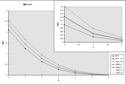
The results are presented in tabular form in Tables 1 and 2, and graphically, for NBO, in Figure 3. The “Poissonification” of the aggregate demand process predicted, or rather stated, by Drenick’s theorem is evident in the results. The NBO and ROS values are extremely insensitive to the underlying distribution assumed for the sub-processes. When comparing with a 10% error in the mean demand rate (see Figure 3) it is obvious that our efforts should be spent on establishing reliable means rather than searching component failure distributions.
What if there are only 30 processes superposed? Let us look at a second case which is in essence identical to the first case except that there are now 30
subprocess-NBO
S exp exp -10% exp +10% W(2) W(4) U(0.5) U(0.2)
1 1.455 1.247 1.667 1.455 1.456 1.457 1.457
2 0.781 0.626 0.947 0.779 0.779 0.781 0.780
3 0.361 0.268 0.469 0.357 0.357 0.358 0.358
4 0.145 0.0988 0.203 0.141 0.141 0.141 0.141
5 0.0507 0.0316 0.0770 0.0479 0.0478 0.0480 0.0481
6 0.0157 0.00891 0.0259 0.0142 0.0142 0.0144 0.0145
Table 1: Expected number of backorders, 100 processes superposed
ROS
S exp exp -10% exp +10% W(2) W(4) U(0.5) U(0.2)
0 1.000 1.000 1.000 1.000 1.000 1.000 1.000
1 0.906 0.882 0.926 0.906 0.907 0.907 0.906
2 0.686 0.631 0.735 0.686 0.686 0.686 0.686
3 0.426 0.363 0.487 0.423 0.423 0.423 0.423
4 0.219 0.171 0.270 0.214 0.214 0.214 0.214
5 0.0947 0.0676 0.127 0.0902 0.0899 0.0901 0.0904
6 0.0351 0.0228 0.0514 0.0323 0.0322 0.0323 0.0327
Table 2: Risk of shortage, 100 processes superposed
NBO vs S
0 0.5 1 1.5 2 2.5 3
0 1 2 3 4 5 6
S
NBO
EXP
EXP -10%
EXP +10%
WEIB(2)
WEIB(4)
UNIF(0.5)
UNIF(0.2) 0
0.02 0.04 0.06 0.08 0.1 0.12 0.14 0.16 0.18 0.2
4 4.5 5 5.5 6
S
NBO
Figure 3: Expected number of backorders, 100 processes superposed. Note how the
curves, except for exp -10% and exp +10%, basically coincide
NBO
S exp exp -10% exp +10% W(2) W(4) U(0.5) U(0.2)
1 1.382 1.192 1.575 1.381 1.381 1.382 1.381
2 0.746 0.602 0.899 0.737 0.738 0.738 0.734
3 0.347 0.259 0.448 0.333 0.332 0.332 0.327
4 0.140 0.0957 0.195 0.126 0.125 0.125 0.122
5 0.0493 0.0307 0.0745 0.0402 0.0396 0.0396 0.0388
6 0.0154 0.00874 0.0253 0.0109 0.0106 0.0106 0.0104
Table 3: Expected number of backorders, 30 processes superposed
ROS
S exp exp -10% exp +10% W(2) W(4) U(0.5) U(0.2)
0 1.000 1.000 1.000 1.000 1.000 1.000 1.000
1 0.900 0.876 0.920 0.900 0.900 0.900 0.900
2 0.677 0.622 0.725 0.673 0.672 0.670 0.672
3 0.419 0.357 0.478 0.406 0.406 0.410 0.402
4 0.215 0.168 0.265 0.198 0.197 0.200 0.193
5 0.0930 0.0664 0.125 0.0780 0.0772 0.0770 0.0760
6 0.0346 0.0224 0.0507 0.0256 0.0249 0.0249 0.0245
Table 4: Risk of shortage, 30 processes superposed
NBO vs S
0 0.5 1 1.5 2 2.5
0 1 2 3 4 5 6
S
NBO
EXP EXP -10% EXP +10% WEIB(2) WEIB(4) UNIF(0.5) UNIF(0.2) 0
0.02 0.04 0.06 0.08 0.1 0.12 0.14 0.16 0.18 0.2
4 5 6
S
NBO
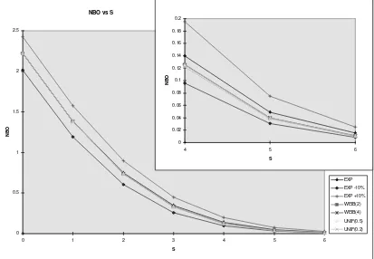
Figure 4: Expected number of backorders, 30 processes superposed Note how the
curves, except for exp, exp -10% and exp +10%, basically coincide
The results are presented in tabular form in Tables 3 and 4, and graphically, for NBO, in Figure 4. The “Poissonification” has not prevailed to the same extent as in the previous case. Nonetheless, a 10% error in the mean demand rate (see Figure 4) has a greater impact on NBO than component failure distribution for all distributions analyzed.
How many component failure processes are involved when forming spares de-mand for an item at a site? Of course, there is no general answer to this question. As we have argued in this paper there are normally many due to several forms of multi-plicity. There are often several systems supplied (directly or indirectly) from a stock. There are often several copies of the item per system. And, perhaps most importantly, there are several components in each item that can fail and generate a spare demand for the item.
7.
Conclusions
The purpose of this paper has been to show that assuming constant demand rates is not the same as assuming constant failure rates. Furthermore, we have motivated why
demand processes for spares tend to be (or are well-approximated by) Poisson proc-esses, although the underlying failure processes for components need not be. The theoretical foundation has been limit theorems for superposition of processes by Drenick and Khintchine. By simulation we have illustrated what happens in the finite case, that is, when a finite number of processes are superposed.
Taking into account the general difficulty in establishing parameter certainty, the simulation examples illustrate the futility in building “more accurate” models on un-certain data. The actual component failure distributions normally have far less impact on spares requirements than the mean demand rate.
Furthermore, we have pointed out that renewal processes lack several beneficial properties of Poisson processes. The lack of closedness under superposition, for ex-ample, is definitely a huge obstacle when trying to model echelon, multi-indenture systems.
References
[Cho96] Chorley, E.P., The Value of Field Data and its Use in Determining Critical Logistic Support Resources, Proceedings of the 6th International MIRCE Symposium, Exeter, UK, 1996, pp.18–32.
[Cox62] Cox, D.R., Renewal Theory, Methuen & Co, London, 1962.
[Cro96] Crocker, J., Weibull Parameter Estimation – A Comparison of Methods, Proceedings of the 6th International MIRCE Symposium, Exeter, UK, 1996, pp. 35–51
[Gra85] Graves, S.C., A Multi-Echelon Inventory Model for a Repairable Item with One-for-one Replenishment, Management Science, Vol 31, 1985, pp. 1247–1256.
[HW63] Hadley, G., and Whitin, T.M., Analysis of Inventory Systems, Prentice-Hall, Englewood Cliffs, 1963.
[Isd99] Isdal T.G., Dynamic Spares Allocation, Proceedings of the 15th Interna-tional Logistics Congress, Exeter, UK, 1999, pp.104–115.
[Khi60] Khintchine A.J., Mathematical Methods in the Theory of Queueing, Charles Griffin & Co, London, 1960.
[Muc73] Muckstadt J.A., A Model for a Item, Echelon,
Multi-Indenture Inventory System, Management Science, Vol 20, 1973, pp. 472– 481
[Pal38] Palm C., Analysis of the Erlang Traffic Formula for Busy-Signal Ar-rangements, Ericsson Technics, Vol 5, 1938, pp. 39–58.
[She68] Sherbrooke C.C., METRIC: A Multi-Echelon Technique for Recoverable Item Control, Operations Research, Vol 16, 1968, pp. 122–141.
[She86] Sherbrooke C.C., VARI-METRIC: Improved Approximation for Multi-Indenture, Multi-Echelon Availability Models, Operations Research, Vol 34, 1986, pp. 311–319.