UAV-based photogrammetry: monitoring of a building zone
J. Unger, M. Reich, C. Heipke
Institute of Photogrammetry and GeoInformation, Leibniz Universität Hannover, Germany - [email protected]
KEY WORDS: UAV, sensor orientation, DEM generation, empirical investigation, software comparison
ABSTRACT:
The use of small-size unmanned aerial vehicles (UAV) for civil applications in many different fields such as archaeology, disaster monitoring, aerial surveying or mapping has significantly increased in recent years. The high flexibility and the low cost per acquired information compared to classical systems – terrestrial or aerial – offer a high variety of different applications. This paper addresses the photogrammetric analysis of a monitoring project and gives an insight into the potential of UAV using low cost sensors and present-day processing software. The area of interest is the “zero:e-park”, a building zone of zero emission housing in Hannover, Germany, that we monitored in three different epochs over a period of five months. We show that we can derive three dimensional information with an accuracy of a few centimetres. Changes during the epochs, also small ones like the dismantling of scaffolding can be detected. We also depict the limitations of the DEM generation approach which occur at sharp edges and height jumps as well as repetitive structure. Additionally, we compare two different commercial software packages which reveals that some systematic errors still remain in the results.
1. INTRODUCTION
Unmanned Aerial Vehicles (UAV) equipped with a camera offer the possibility to map distinct regions fast and with high flexibility compared to classical aerial photogrammetry. With a ground sampling distance (GSD) at a level of a few centimetres UAV can be used for various tasks such as 3D object reconstruction, producing digital elevation models (DEM) and orthophotos (Remondino et al. 2011; Haala et al. 2013). The results can be used for inspection of industrial facilities, mapping of archaeological or agricultural sites, disaster monitoring, mapping, etc. With the possibility to operate at small flying heights and with different viewing directions UAVs can be said to close the gap between terrestrial and classical aerial photogrammetry.
In this paper we analyse and compare the results of a photogrammetric monitoring project. The area we work in is the “zero:e-park” in Hannover, Germany, at present Europe’s largest building zone of zero-emission housing. Our region of interest spans an area of approximately 350x450m2 (figure 1); using UAV for that purpose offers the possibility to acquire relevant data within a high temporal frequency. However, the automatic processing of the data exhibits a number of challenges for present-day software solutions. Firstly, compared to classical aerial photogrammetry the flight pattern is not as regular which results in a higher variation of the rotation parameters. Secondly, due to the limited payload the employed imaging sensor and lens often have a rather low quality leading to blurry and noisy imagery. To analyse the potential of UAV photogrammetry for our purposes we acquired three datasets of the building zone at three epochs within five months. We processed each epoch separately using the commercial software package PhotoScan Professional1 of Agisoft. For the comparison of different epochs the results are oriented using ground control points (GCP) measured by real time kinematic GPS. Hence, we are able to detect geometrical changes between different epochs which can be visually interpreted using derived orthophotos.
1
http://www.agisoft.ru/products/photoscan/professional/
Furthermore, we compare the solutions of one epoch with an additional self-contained software package, namely Pix4D’s commercial software Pix4DMapper2.
Figure 1: Orthophoto of the zero:e-park acquired in the monitoring campaign (processed by PhotoScan)
2. RELATED WORK
An extensive overview of the evolution and the state-of-the-art of photogrammetry and remote sensing using UAV is given by Colomina and Molina (2014). The authors describe early developments and present a literature review on UAVs for photogrammetry and remote sensing covering topics like flight regulation, navigation, orientation, sensing payloads and data processing. Furthermore applications and geomatic markets are outlined.
Gini et al. (2013) compare two traditional digital photogrammetric software packages to Pix4UAV (the
2
http://pix4d.com/products/
predecessor of Pix4DMapper) and PhotoScan that where specifically designed for handling UAV images. The authors conclude that in their investigation these packages found more tie points and provided a higher rate of automation compared to the traditional software. Concerning the DSMs PhotoScan is reported to achieve the most reliable results.
Remondino et al. (2012) investigate automated image orientation packages including APERO (a sub module of the open source software MicMac, dealing with orientation; Deseilligny and Clery (2011)) and PhotoScan using terrestrial and aerial datasets with up to 212 images. The comparison of the software packages is done visually for internal and external orientation parameters, by shapes and distances or by a network of GCPs (4 GCP, 20 check points).
In our work we deal with a large amount of images (>1000 per epoch) which leads to higher complexity in data processing and constitutes a certain challenge for present-day software packages. Furthermore, we demonstrate the use of UAVs for the purpose of photogrammetric monitoring of rather small areas compared to classical aerial photogrammetry. Our goal is to reach a ground resolution of a few centimetres and an accuracy of the 3D reconstruction below 5cm using low-cost cameras and a UAV with a payload limited to a few hundred g.
3. PRELIMINARIES
3.1 Hardware
In the project we used a Microdrones md4-200 micro-UAV vertical take-off and landing (VTOL) quadrocopter equipped with low-cost GPS and IMU. It has a maximum payload of 200g, hence we are highly limited in possible imaging devices. In our experiments we used two different sensors: the Canon IXUS 100IS and the slightly heavier but more powerful PowerShot S110; in both cases we only capture vertical images. The PowerShot has a larger sensor allowing shorter exposure time and a shorter focal length leading to a wider viewing angle (see table 1 for details). A shorter exposure time helps to reduce blurring in the captured images caused by vibrations and the movement of the UAV. The wider viewing angle leads to higher overlap of the images under otherwise identical conditions. An automatic data capture is achieved using the Canon Hack Development Kit (CHDK)3 in which a script mode enables capturing images based on a predefined time interval.
3.2 Ground Control and Check Points
We used the centre of man hole covers as GCPs because their appearance in the image allows a reliable manual determination of the centre. In total object coordinates of 33 points were
The flight was planned using the Microdrones tool mdCockpit. According to the requirements mentioned above, the flying height was set to 60m above ground leading to a GSD between 1.7cm and 3cm depending on the camera and the used image resolution. To obtain the maximum possible flying speed, we evaluated the minimum time interval between capturing two images using full resolution which turned out to be around two
3
http://chdk.wikia.com/wiki/CHDK
seconds. Fixing the flying velocity at 2.5m/s resulted in an image overlap of around 84 or 89% within the strip; the side overlap was 73 or 80% depending on the camera (table 1). Due to the limited battery capacity the grid based flight plan had to be subdivided into 5 flights per epoch, these were flown processing. Blurred images were excluded from further calculations manually. Images captured with the PowerShot with an exposure time between 1/1600s and 1/2000s showed significantly less blur than the IXUS-images captured at 1/1000s. Using the PowerShot, 99% of the images revealed a sufficient quality.
4.1 Bundle Adjustment
Next, the usual photogrammetric workflow for each epoch was carried out using PhotoScan. We first determined initial values for the projection centres from the log-data of the UAV. Subsequently, we manually measured the image coordinates of the GCPs and check points. The next step was automatic matching of tie points which is done using a feature based approach. The resulting tie point coordinates were used as observations in a robust bundle adjustment. The parameters of the interior orientation of the camera were calculated by self-calibration within the bundle adjustment process. The accuracy of the object coordinates of the GCPs was set to 2cm.
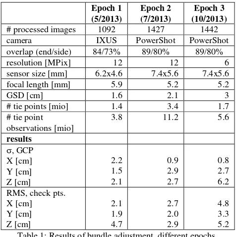
Epoch 1
camera IXUS PowerShot PowerShot
overlap (end/side) 84/73% 89/80% 89/80% Table 1: Results of bundle adjustment, different epochs
Table 1 lists the configuration of the three epochs, the standard deviations at the GCPs and the root mean square (RMS) values of the check points. The results appear to be reasonable taking into account that RTK-GPS provides an accuracy of 2cm and the fact that the GSD is at the same level. Furthermore, the standard deviations of GCPs and RMS values of the check points are rather similar and hence reveal realistic results. The International Archives of the Photogrammetry, Remote Sensing and Spatial Information Sciences, Volume XL-5, 2014
However, in epochs 1 and 3 some points near the boundary of the region have high Z-residuals (up to 9cm) explaining the higher RMS values. In addition the images in epoch 3 were acquired with a coarser GSD of 3cm and some of the images were acquired with fog in the air.
To further analyse the bundle adjustment results we investigated the residuals of the GCPs and the check points. Figure 2 shows the plot for the planimetric residuals of the second epoch. The blue check point deviations and also the red GCP deviations at certain regions have similar directions, which can be interpreted as systematic effects remaining in the results. The Z-residuals (not depicted here) also indicate systematic deviations. Additionally, one can observe that the highest residuals are found on the eastern side (up to 7 cm in planimetry). A possible reason for this is that they are close to the border of the observed region and hence covered by fewer images.
Figure 2: Residuals at GCPs (red) and check points (blue) and their distribution over the building zone for the second epoch
(projected onto XY-plane)
4.2 Point Cloud, DSM and Orthophoto
The next processing step is the densification of the sparse 3D point cloud of tie points by dense matching. The resulting dense point cloud is then used to derive a digital surface model (DSM) and an orthophoto of the whole scene.
We analysed changes between the epochs in the observed scene by subtracting DSMs, visualising changes in height and comparing them to corresponding orthophotos for interpretation purposes.
Figure 3 shows the height changes between -10m and 10m for the whole 5 months period. Areas depicted in green showed an increase in height, whereas red means a height decrease. For example, one can see where scaffoldings around buildings where dismantled (linear red lines around buildings), where parts of buildings were constructed and where ground was moved (tender red areas). These observations have been verified by consulting the corresponding orthophotos. One can clearly see that there was more building activity on the eastern part of the area while there was detailed work on already constructed buildings in the west.
Figure 3: DSM difference between 1st and 3rd epoch (5 months)
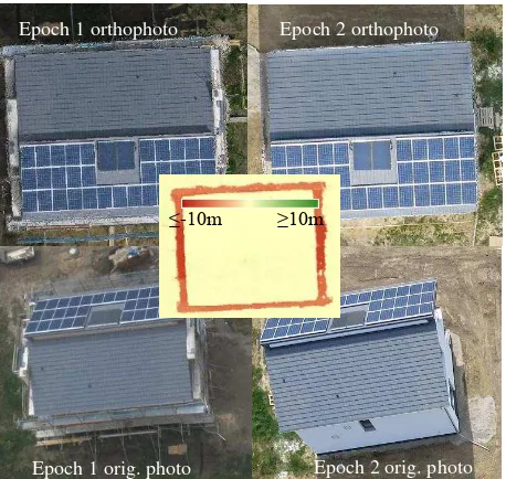
The following examples show details that can be seen in the images and the possibilities of our monitoring approach. Figure 4 relates the height decrease around a building that is seen in the DSM difference to the corresponding orthophotos and one of the aerial images of each epoch. In the first epoch there was a scaffolding around the building while it was dismantled in the second one.
Figure 4: Dismantled scaffolding around a building
Figure 5 demonstrates the possibility of observing earth mass movements. The pile of earth visible in the first epoch was distributed over the area before the images to the second epoch were taken.
≤-10m ≥10m
Epoch 1 orthophoto Epoch 2 orthophoto
Epoch 1 orig. photo Epoch 2 orig. photo
≤-10m ≥10m 7cm
Figure 5: Earth mass movement
Figure 6 shows a building that was shifted between the epochs. As confirmed by the owners, this shift in object space (!) was necessary, since the original location was wrong due to some planning error.
Figure 6: Shifted building
These examples show the potential of this approach for precise computations of volumetric changes that are of high value in many different fields. However, when using the results one should be aware of possible problems which are demonstrated in the following.
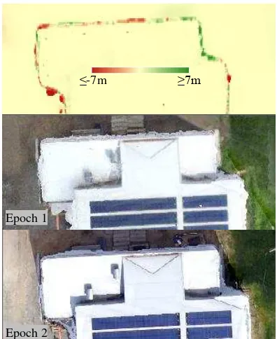
Examples for possibly unwanted height-differences in the model are movable objects like cars, containers and people in the scene. More important are height-differences that don’t exist in the scene and stem from image matching problems. Buildings in general lead to sudden height changes from roof to ground. It is well known that these height jumps are difficult to reconstruct, also in dense matching. The flatness of the model highly depends on the dense matching algorithm, more precisely on the weighting between the data term and the smoothness constraint. This may lead to different smoothing at the building outlines. The result is a small (~20cm) erroneous boundary in the DSM difference between two epochs. Figure 7 shows an example for a house that did not change between two epochs and hence should have no difference in the DSM difference (note the relatively large derived height difference).
Another effect we observed in the DSM difference using PhotoScan depends on the so called dense matching “mode”, which affects the level of detail of this processing step. Figure 8 shows DSMs and orthophotos of the same epoch computed with different modes. In “high”-mode (upper part) the reconstruction of the roof was unsuccessful while in “medium” (lower part) the roof is approximately a plane and leads to a correct orthophoto.
Figure 7: Sudden height changes in between epochs for stable objects
Figure 8: Errors depending on dense matching mode ≤-1m ≥1m
≤-7m ≥7m
≤-7m ≥7m
Epoch 2 DSM in “high” dense matching mode
Epoch 2 DSM in “medium” dense matching mode
Epoch 2 ortho in “high” dense matching mode
Epoch 2 ortho in “medium” dense matching mode
Epoch 1 Epoch 2
120m
100m Epoch 2
Epoch 1
Epoch 2 Epoch 3
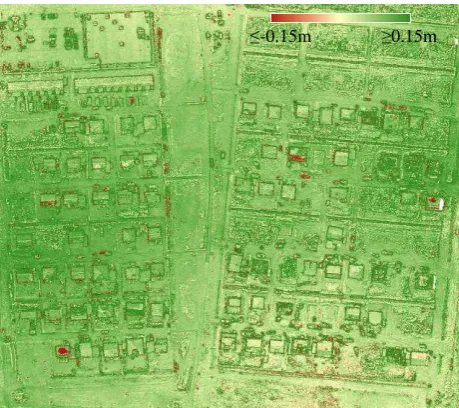
To analyse also the repeatability of our work we investigated areas in the DSMs which manifest themselves in a rather flat appearance (e. g. car parks, roofs, solar panels): we looked at differences in height. The difference of the DSMs over time in those areas should be zero. Figure 9 shows the DSM difference between epochs 2 and 3 in the range of -15cm to 15cm, where black depicts differences above respectively below this range. We are interested in changes in centimetre range which reveal an erroneous global tilt or even oscillations in the scene. While in the central eastern part streets and roofs of unchanged buildings show increased height (reddish colour), in the north-western part and in the south one can observe decreased height of such areas (greenish colour). These height changes are systematic and larger than they normally should be e.g. due to dust on the roads. We therefore conclude that there are systematic effects left that are probably the result of the systematic effects we already observed in the GCP and check point residuals (see Figure 2). Such effects occur also between the first and the second epoch.
Figure 9: DSM difference between 2nd and 3rd epoch in centimetre range (-15cm to 15cm)
5. SOFTWARE COMPARISON
In this chapter we report on a comparison of the two mentioned software packages, in particular the bundle adjustment results, the point clouds and the orthophotos delivered by PhotoScan and Pix4DMapper. We used the same imagery and the same image coordinates of the GCPs and check points in both software packages. In doing so we provide an analysis based on comparable conditions. The GPS positions of the projection centres are used only as initial values in the bundle adjustment and to accelerate the matching and orientation process. The comparison of the two software packages is done for epoch 2 only. The bundle adjustment results are compared using remaining discrepancies in the GCP and check point coordinates (table 2).
As can be seen the number of tie points and observations in Pix4DMapper was found to be significantly higher than in PhotoScan. Furthermore, the residuals of the GCPs are more homogeneous and smaller in X, Y and Z. Nevertheless, the RMS values of the check points are somewhat larger than those of the GCPs which leads to the fact, that the model is fitted more strongly to the GCPs than in PhotoScan.
Epoch 2 Pix4DMapper PhotoScan
# tie points [mio] 5.6 3.4
# tie point observations [mio]
21.2 11.2
, GCP X [cm] Y [cm] Z [cm]
1.0 1.2 1.1
0.9 2.9 2.7 RMS,check pts.
X [cm] Y [cm] Z [cm]
2.1 1.0 2.0
2.7 2.0 2.9 Table 2: Results of bundle adjustment, different software
packages
To further analyse these results, we also looked at the residuals of GCPs and check points for Pix4DMapper (figure 10). The residuals of the check points have no obvious remaining systematic effects. The same applies for the Z-residuals.
Figure 10: Residuals at GCPs (red) and check points (blue) and their distribution over the building zone for the second epoch
processed with Pix4DMapper (projected onto XY-plane)
Figure 11: DSM difference of the second epoch between Pix4DMapper and PhotoScan in centimetre range (-15cm to
15cm)
To investigate the geometric quality of the 3D reconstruction we compare DSMs. Figure 11 shows the result for the comparison between PhotoScan and Pix4DMapper which again reveals some systematic effects. The Pix4DMapper DSM was subtracted from the one computed by PhotoScan. Especially in
≤-0.15m ≥0.15m >-0.15m <0.15m
6cm The International Archives of the Photogrammetry, Remote Sensing and Spatial Information Sciences, Volume XL-5, 2014
the central western and eastern part the PhotoScan DSM clearly lies above the one derived with Pix4DMapper. As we did not see any systematic effects in Pix4DMappers residuals this can be interpreted such that the systematic effect visible in the DSM difference is caused by PhotoScan.
As we already mentioned, sudden height changes are a challenge in matching. In the software comparison we observed a larger problematic boundary around building edges for Pix4DMapper (figure 12) compared to PhotoScan. This is shown for the DSMs and for the resulting orthophotos and is valid for the majority of the buildings in our scene. While edges are generally sharper in the PhotoScan results, for some buildings artefacts of the roof edge are visible (see at the bottom of the PhotoScan orthophoto in figure 12).
Figure 12: DSM difference PhotoScan minus Pix4DMapper and corresponding orthophotos and DSMs
6. CONCLUSION
Our investigations show that UAVs are a cost and time efficient alternative to classical aerial photogrammetry for mapping and monitoring small areas. High resolution and, with some limitations, high accuracy products can be generated and used for change detection. Small changes like the dismantling of scaffoldings are visible in DSM differences. Limitations of the approach have been found and were depicted using examples. This accounts for some remaining systematic effects during image orientation and for properly representing height jumps during image matching.
While Pix4DMapper seems to perform better in bundle adjustment, PhotoScan shows fewer problems in dense matching and orthophoto generation. The accuracy at check
points reported by Pix4DMapper reaches the level that one would expect in classical aerial photogrammetry with the same flight parameters.
We plan to further investigate the systematic effects left in the bundle adjustment results and the problems in the quality of the DSMs and orthophotos with additional scenes and other flight configurations.
General limitations of UAV photogrammetry are wind conditions, payload, battery and legal restrictions. The used UAV is limited to a wind speed of up to 30km/h. With the PowerShot camera we reached the maximum payload and we hardly reached 15 minutes of flight time with one battery.
ACKNOWLEDGEMENTS
We thank our students for their assistance: Zhouran Cao, Yu Feng, Ayşe Şahin, Leonard Hiemer, Niklas Kläve and Christoph Wallat.
REFERENCES
Colomina, I., Molina, P., 2014. Unmanned Aerial Systems for Photogrammetry and Remote Sensing: A Review. ISPRS Journal of Photogrammetry and Remote Sensing 92: 79– 97. 10.1016/j.isprsjprs.2014.02.013.
Deseilligny, M. P., Clery, I., 2011. Apero, an open source bundle adjustment software for automatic calibration and orientation of set of images. Proceedings of the ISPRS Symposium, 3DARCH11: 269–277.
Gini, R., Pagliari, D., Passoni, D., Pinto, L., Sona, G., Dosso, P., 2013. UAV Photogrammetry: Block Triangulation Comparisons. ISPRS - International Archives of the Photogrammetry, Remote Sensing and Spatial Information Sciences XL-1/W2: 157–162. 10.5194/isprsarchives-XL-1-W2-157-2013.
Haala, N., Cramer, M., Rothermel, M., 2013. Quality of 3D Point Clouds from Highly Overlapping UAV Imagery. ISPRS - International Archives of the Photogrammetry, Remote Sensing and Spatial Information Sciences XL-1/W2: 183–188. 10.5194/isprsarchives-XL-1-W2-183-2013.
Remondino, F., Barazzetti, L., Nex, F., Scaioni, M., Sarazzi, D., 2011. Uav Photogrammetry for Mapping and 3D Modeling – Current Status and Future Perspectives. ISPRS - International Archives of the Photogrammetry, Remote Sensing and Spatial Information Sciences XXXVIII-1/C22: 25–31.
Remondino, F., Pizzo, S., Kersten, T. P., Troisi, S., 2012. Low-Cost and Open-Source Solutions for Automated Image Orientation – A Critical Overview. In: Hutchison, D., Kanade, T., Kittler, J., Kleinberg, J. M., Mattern, F., Mitchell, J. C., Naor, M., Nierstrasz, O., Pandu R., C., Steffen, B., Sudan, M., Terzopoulos, D., Tygar, D., Vardi, M. Y., Weikum, G., Ioannides, M., Fritsch, D., Leissner, J., Davies, R., Remondino, F., Caffo, R. Progress in Cultural Heritage Preservation, 40–54. Berlin, Heidelberg: Springer Berlin Heidelberg.
Epoch 2 ortho and DSM by PhotoScan
Epoch 2 ortho and DSM by Pix4DMapper
≤-7m ≥7m
120m
95m