MULTI-YEAR GLOBAL LAND COVER MAPPING AT 300 M AND
CHARACTERIZATION FOR CLIMATE MODELLING: ACHIEVEMENTS OF THE
LAND COVER COMPONENT OF THE ESA CLIMATE CHANGE INITIATIVE
S. Bontemps a,*, M. Boettcher b, C. Brockmann b, G. Kirches b, C. Lamarche a, J. Radoux a, M. Santoro c, E. Van Bogaert a, U.Wegmüller c, M. Herold d, F. Achard e, F. Ramoino f, O. Arino f, P. Defourny a
a
Université catholique de Louvain, Earth and Life Institute, Belgium - (Sophie.Bontemps, Céline.Lamarche, Julien.Radoux, Eric.Vanbogaert, Pierre.Defourny)@uclouvain.be
b
Brockmann Consult GmbH, Hamburg, Germany - (Martin.Boettcher, Carsten.Brockmann, Grit.Kirches)@brockmann-consult.de c
Gamma Remote Sensing, Switzerland – (santoro, wegmuller)@gamma-rs.ch d Wageningen University, the Netherlands – [email protected]
e
Joint Research Centre, Italy – [email protected] f
European Space Agency, European Space Research Institute, Italy – (Fabrizio.Ramoino, Olivier.Arino)@esa.int
KEY WORDS: Land Cover, Global, Time Series, Consistency, Essential Climate Variable
ABSTRACT:
Essential Climate Variables were listed by the Global Climate Observing System as critical information to further understand the climate system and support climate modelling. The European Space Agency launched its Climate Change Initiative in order to provide an adequate response to the set of requirements for long-term satellite-based products for climate. Within this program, the CCI Land Cover project aims at revisiting all algorithms required for the generation of global land cover products that are stable and consistent over time, while also reflecting the land surface seasonality. To this end, the land cover concept is revisited to deliver a set of three consistent global land cover products corresponding to the 1998-2002, 2003-2007 and 2008-2012 periods, along with climatological 7-day time series representing the average seasonal dynamics of the land surface over the 1998-2012 period. The full Envisat MERIS archive (2003-2012) is used as main Earth Observation dataset to derive the 300-m global land cover maps, complemented with SPOT-Vegetation time series between 1998 and 2012. Finally, a 300-m global map of open permanent water bodies is derived from the 2005-2010 archive of the Envisat Advanced SAR imagery mainly acquired in the 150m Wide Swath Mode.
* Corresponding author
1. INTRODUCTION
The demand for information on climate has never been greater than today (GCOS, 2010; IPCC, 2014). In 2004, the Global Climate Observing System (GCOS) established a first list of Essential Climate Variables (ECV), selected to be critical for a full understanding of the climate system and currently ready for global implementation on a systematic basis (CEOS, 2008).
In this context, the European Space Agency (ESA) initiated a new program of ECV global monitoring – known for convenience as the Climate Change Initiative (CCI) – which aims at providing a comprehensive and timely response to the need for long-term satellite-based products in the climate domain (ESA, 2009). The ESA-CCI program focuses, through individual projects, on 13 ECVs selected in the atmospheric, oceanic and terrestrial domains. The selection was driven by GCOS demands and the capabilities of ESA space mission. One project is dedicated to land cover. Land cover is indeed referred to as one of the most obvious and commonly used indicators for land surface and the associated human induced or naturally occurring processes, while also playing a significant role in climate forcing (Herold et al., 2009).
The overall objective of the CCI Land Cover (CCI-LC) project is to critically revisit all algorithms required for the generation of a global land cover product in the light of GCOS requirements, to be generated from data of various Earth
Observation (EO) instruments and matching the needs of key users belonging to the climate modelling community.
2. CLIMATE MODELLING COMMUNITY CONSULTATION
During the six first months of the project, a user requirements analysis was conducted to derive the specifications for a new global Land Cover (LC) product to address the needs of key-users from the climate modelling community. The objective was twofold: (i) understand how LC data were used by the modellers and (ii) identify the future expectations for LC data in the context of climate and Earth system modelling. This user assessment was built upon the general guidance from the GCOS and its related panel activities and provided the next step to further derive more detailed characteristics and foundations to observe LC as an ECV.
it still counts more than 500 hits by week on the project webpage (http://due.esrin.esa.int/page_globcover.php). In addition, a detailed literature review was carried out with special attention to innovative concepts and approaches to better reflect land dynamics in the next generation climate models.
Figure 1. User consultation mechanism established to assess LC requirements. Percentages indicate the number of responses
received from each user’s group
This consultation showed that although the range of requirements coming from the climate modelling community is broad, there was a good match among the requirements coming from different user groups and the broader requirements derived from international organizations. Detailed user requirements assessment can be found in Herold et al. (2011). One finding of particular interest was the need for successive LC products stable over time (i.e. free from any temporary variability). In climate models, LC maps are indeed often used as a consistent basis for land surface parameterization and thus need to be stable to avoid – as much as possible – introducing inconsistencies in model inputs.
3. A NEW LAND COVER CONCEPT
The users’ requirements analysis highlighted expectations for an improved LC product which would be more integrative than the current one. Indeed, there was a clear requirement for a land cover which includes both stable and dynamic components, while making the difference between LC change and natural variability.
The existing suite of global LC products doesn’t meet this requirement: successive annual LC maps are contaminated by significant inter-annual variations, due to phenology and disturbances rather than to LC changes (Bontemps et al., 2009; Friedl et al., 2010). As a result, the whole LC concept was revisited with the aim of defining two distinct products to represent the stable and dynamic components of the land surface (Defourny and Bontemps, 2012).
On one hand, global LC maps should refer to the set of LC features remaining stable over time which define the LC independently of any sources of temporary or natural variability. On the other hand, a complementary product should be generated to describe the temporary or natural variability of LC features that can induce some variation in land surface over time without changing the LC in its essence. This second product could encompass different observable variables such as the green vegetation phenology, snow coverage, open water presence, burned areas occurrence, etc.
From the remote sensing point of view, the global LC maps should be derived from multi-year observation datasetto reduce the sensitivity of the classification methods to the date(s) of observation (Bontemps et al., 2012). Conversely, the natural variability of the land surface has to be considered within the perspective of a time cycle (typically a year) precisely in order to reflect the above-mentioned temporary conditions.
4. A NEW GENERATION OF GLOBAL LAND COVER PRODUCTS
Based on this innovative result, the CCI-LC project delivered in October 2014 global LC databases made of LC maps at 300m spatial resolution for three 5-year epochs – centred around 2000, 2005 and 2010 – and of land surface seasonality products. The surface reflectance (SR) time series which served as input for generating the global LC databases were also delivered as CCI-LC products. In addition, a 300-m global map of open permanent water bodies was derived from the 2005-2010 archive of the Envisat Advanced SAR (ASAR) imagery mainly acquired at 150m.
4.1 Surface reflectance time series
The main source of input EO data for the global LC maps is the full archive (2003-2012) of MERIS instrument.
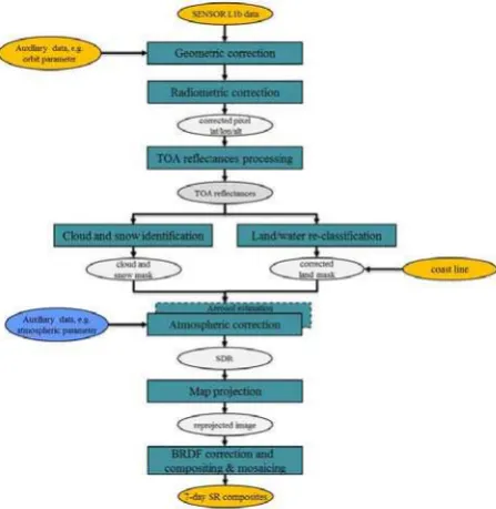
The MERIS Full and Reduced resolution (FR and RR respectively - 300m and 1000m) time series are pre-processed in the framework of the project. The completed automated pre-processing chain performs the following operations (Figure 2): radiometric, geometric correction, identification of water/snow/cloud/cloud shadow/invalid pixels, atmospheric correction with aerosol retrieval as well as compositing and mosaicking. The output time series are made of temporal syntheses obtained over a 7-day compositing period (Figure 3).
Figure 2. Schematic representation of the CCI-LC pre-processing chain (based on GlobAlbedo project, 2013)
13 of 15 MERIS spectral channels, bands 11 and 15 being removed.
Figure 3. Example of SR 7-day composite, at 300m spatial resolution generated in the CCI-LC project
4.2 Global land cover maps
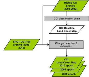
In order to meet the requirement to have successive global LC maps stable over time (see section 2), several years of EO dataset are used to generate each global LC map. This is the reason why the project delivers maps which are not related to single years but which are representative of 5-year epochs: 1998-2002, 2003-2007 and 2008-2012. Furthermore, these 3 maps are not derived independently but from a unique “baseline” LC map generated using the full MERIS archive (i.e. 10 years of data from 2003 to 2012). This “baseline” LC map is then back- and up-dated using a change detection approach based on SPOT-VGT time series. The whole workflow is presented in Figure 4.
Figure 4. Classification workflow developed to generate global LC maps stable over time
The classification chain transforms the MERIS 7-day composites produced by the pre-processing module into meaningful global land cover products in 4 major processing steps. In the first and second steps, both machine learning and
unsupervised classification algorithms are run using the spectral properties of MERIS composites. The 2 first steps result in two different classifications which are then merged in a third step based on objective rules. The fourth step finalizes the “baseline” LC maps through a set of post-classification editions.
The classification process is based on a-priori stratification of the world in equal-reasoning areas from an ecological and a remote sensing point of view. The classification process has been designed to run independently for each delineated equal-reasoning area.
The 3 epochs are then derived from the 10-year MERIS-based “baseline” LC map (Figure 5 and Figure 6). Up to now, only macroscopic forest cover changes have been targeted. Forest changes are identified through a specific analysis of successive annual classifications of SPOT-VGT time series (1998-2012). The changes identified at the SPOT-VGT 1km resolution are then re-mapped at the MERIS 300m resolution in the corresponding epoch (Figure 6).
The typology is made of 22 classes defined using the UN Land Cover Classification System (Di Gregorio, 2005) with the view to be as much as possible compatible with the GLC2000, GlobCover 2005 and 2009 products (Table 1). This system has been found quite compatible with the Plant Functional Types used by most climate modellers (Herold et al. 2011).
Label Color
No Data Cropland, rainfed
Cropland, irrigated or post-flooding
Mosaic cropland (>50%) / natural vegetation (<50%) Mosaic natural vegetation (>50%) / cropland (<50%) Tree cover, broadleaved, evergreen, closed to open Tree cover, broadleaved, deciduous, closed to open Tree cover, needleleaved, evergreen, closed to open Tree cover, needleleaved, deciduous, closed to open Tree cover, mixed leaf type (broadleaved and needleleaved)
Mosaic tree and shrub (>50%) / herbaceous (<50%) Mosaic herbaceous (>50%) / tree and shrub (<50%) Shrubland
Grassland
Lichens and mosses
Sparse vegetation (tree, shrub, herbaceous) (<15%) Tree cover, flooded, fresh or brakish water Tree cover, flooded, saline water
Shrub or herbaceous cover, flooded, fresh/saline/brakish water
Urban areas Bare areas Water bodies
Permanent snow and ice
Table 1. Legend of the global LC maps, based on UN-LCCS
Figure 5. The global CCI-LC map from the 2010 epoch (2008-2012)
Figure 6. The CCI global land cover maps at 300m spatial resolution from the 2010, 2005 and 2000 epochs, over part of
the Amazon basin
The accuracy of the 2008-2012 global LC map was assessed using the GlobCover 2009 validation dataset (Bontemps et al. 2009), resulting in a weighted-area overall accuracy of 74.1% which is slightly better than previous products. In addition, visual analysis revealed a much better delineation of landscape patterns. A more complete validation, based on a global dataset specifically collected within the CCI-LC project, is currently in progress; accuracy figures will be presented at the symposium.
4.3 Global land surface seasonality products
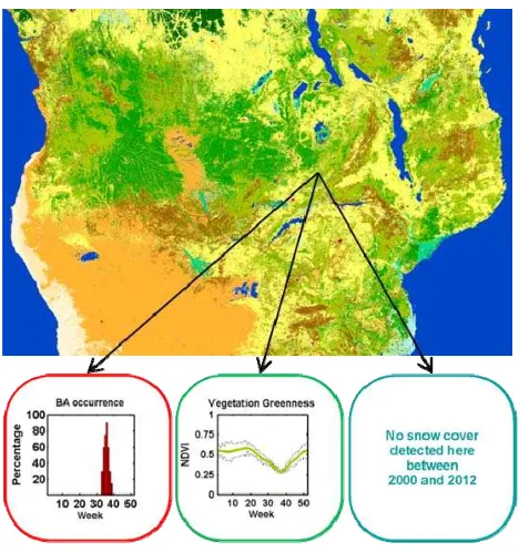
To characterize the typical seasonal dynamics of the land surface at the pixel level, three global climatology products are also generated: the vegetation greenness as described by the Normalized Vegetation Index (NDVI), the snow occurrence and the burned areas distribution over the 1998-2012 period (Figure 7). They are expressed as 7-day time series of the mean and standard deviation for continuous variables (NDVI) or as temporal series of occurrence probabilities for discrete variables (snow and burned areas). Particular emphasis is put on the consistency between these 3 products.
These are compiled from existing global datasets: SPOT-Vegetation daily top of canopy surface reflectance syntheses, the MODIS Direct Broadcast Monthly Burned Area Product being part of the Global Fire Emissions Database version 3 and the 8-day maximum snow extent product for the NDVI, burned areas and snow seasonality products respectively.
Figure 7. Climatological 7-day time series describing consistently and on a per-pixel basis the natural variability of
the vegetation (NDVI), the snow cover and the burned areas
As an example, Figure 8 shows NDVI profiles extracted from 3 pixels belonging to 3 LC classes of the 2010 CCI-LC map. The variety of the dynamic of vegetation is clearly well-captured.
Figure 8. Detailed spatial example of NDVI climatological profiles - mean (plain line) and standard deviation (dotted line)
- extracted in a region of Central Africa.
4.4 Global map of water bodies
Another key output of the project is a global SAR-based Water Bodies (WB) product, which gives the repartition of open and permanent water bodies (inland water and oceans) at 300m spatial resolution and global scale.
Indicator is obtained. Refinements of the WB Indicator are then applied based on visual and inconsistency assessments. The CCI-LC WB product is finally obtained after resampling to the 300m spatial resolution of the global LC maps. Figure 9 gives an example of the thematic precision of the WB product when overlaid on optical imagery.
Figure 9. Detail of the global WB product, showing on left very high spatial resolution imagery from Google Earth and on right
the 300m product
4.5 User tool
The project also delivers a user tool to allow users re-sampling, sub-setting and re-projecting the LC products. Indeed, the LC map and condition products are delivered at a given spatial resolution, all as global files, in a Plate-Carrée projection. However, climate models may need products associated with a coarser spatial resolution, over specific areas (e.g. for regional climate models) and/or in another projection. The developed tool allows them adjusting these three parameters in a way which is suitable to their models.
Furthermore, the tool offers the possibility to couple the aggregation with the conversion from the LC classes expressed using the UN-LCCS to user-specific Plant Functional Types.
5. MODELLING ASSESSMENT
Three different Earth System models respectively from the Laboratoire des Sciences du Climat et l'Environnement (LSCE), the United Kingdom Met Office (MOHC) and the Max Planck Institute (MPI) for Meteorology are adjusted to use as input the new CCI-LC dataset in order to assess the possible simulation improvement against a set of benchmarks. Model experiments include offline as well as coupled carbon-climate simulations, and a dynamic vegetation simulation. For each simulation, the LC maps are converted into Plant Functional Types and merged with climate zones linking with biome specific parameters for structural and physiological traits.
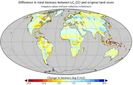
The already obtained results are quite promising. For instance, an initial assessment of the global offline simulations, run by the LSCE with the WATCH-Forcing-Data-ERA-Interim climate forcing from 1979-2009, shows an improvement in modelled aboveground biomass stocks. Most recent forest inventory estimates of total woody biomass are around 363 ±28 Pg C. With the new CCI-LC product, a 56 Pg C reduction in total biomass simulated by ORCHIDEE is found, from 688 to 632 PgC (Figure 10). Much of the reduction in biomass comes from improvements in mapping tropical land cover, where recent land-use transitions due to deforestation processes are included in the CCI-LC dataset but not in the original ORCHIDEE LC dataset.
Figure 10. Difference in total biomass between CCI-LC and original LC products (negative values indicate reduction in
biomass)
Yet, the results obtain by the different climate groups and simulations slightly differ according to the respective models sensitivity. Additional analysis and simulations are in progress to better understand the results and compare the models and datasets.
6. CONCLUSIONS AND NEXT STEPS
In October 2014, the CCI-LC product made the first official release of its five key products: (i) 3 global LC maps at 300m spatial resolution corresponding to the 1998-2002, 2003-2007 and 2008-2012 epochs, (ii) 3 global land cover seasonality products describing the vegetation greenness, the snow and the burned areas occurrence along the year, (iii) a global map of open permanent WB at 300m spatial resolution, (iv) the full archive (2003-2012) of MERIS time series processed in 7-day composites and (v) a user tool for sampling, sub-setting, re-projecting and converting the products into climate model inputs. These products match the needs expressed by the climate research community, but are also of interest for the wider LC community. They can be freely and easily visualize and download online at: http://maps.elie.ucl.ac.be/CCI/viewer.
A second 3-year phase has started now for the project with key objectives: improving the methodologies developed for generating the CCI-LC products, extending in the past and in the future the CCI-LC database, moving to higher spatial resolution.
With respect to the second objective, it is planned to go back to the 1990s (and possibly 1980s) using AVHRR dataset, thus resulting for the first time in a 20 (or 30) year-long LC dataset. The challenge will be to remain consistent with the already existing 2000, 2005 and 2010 global LC maps. To this end, an independent classification is not foreseen.
It is also planned to generate a new global LC map over a 2015 epoch, using the successors of Envisat MERIS and SPOT-VGT, namely Sentinel-3 and PROBA-V.
resolution, with the coming Sentinel-2 coverage of Africa. The contribution of Sentinel-1 to the optical mapping will finally be tested.
REFERENCES
Arendt, A., Bliss, A., Bolch, T., Cogley, J.G., Gardner, A.S., Hagen, J.-O., Hock, R., Huss, M., Kaser, G., Kienholz, G., Pfeffer, W.T., Moholdt, G., Paul, G., Radić, V. et al., 2014. Randolph Glacier Inventory – A Dataset of Global Glacier Outlines: Version 4.0. Global Land Ice Measurements from Space, Boulder Colorado, USA. Digital Media. Available at:
http://www.glims.org/RGI/
Arino, O., Bicheron, P., Achard, F., Latham, J., Witt, R., and Weber, J. L., 2008. Globcover: the most detailed portrait of Earth, ESA Bulletin, 136, pp. 24-31. Available at:
http://www.esa.int/esapub/bulletin/bulletin136/bul136d_arino.p df
Bontemps, S., Defourny, P., Van Bogaert, E., Kalogirou, V. and Arino, O., 2010. GlobCover 2009 - Products Description and Validation Report. Available at:
http://due.esrin.esa.int/files/GLOBCOVER2009_Validation_Re port_2.2.pdf
Bontemps, S., Herold, M., Kooistra, L., van Groenestijn, A., Hartley, A., Arino, O., Moreau, I., and Defourny, P., 2012. Revisiting land cover observations to address the needs of the climate modelling community. Biogeosciences, 9, pp. 2145-2157
CEOS – Committee on Earth Observation Satellites, 2008. The Earth Observation Handbook, Climate Change Special Edition. Available at: http://www.eohandbook.com/eohb2008/
Defourny, P., Bicheron, P., Brockman, C., Bontemps, S., Van Bogaert, E., Vancutsem, C., Pekel, J.F., Huc, M., Henry, C.C., Ranera, F., Achard, F., Di Gregorio, A., Herold, M., Leroy, M. and Arino, O., 2009. The first 300 m global land cover map for 2005 using ENVISAT MERIS time series: A product of the GlobCover system. Proceedings of the 33rd
International Symposium on Remote Sensing of Environment,
pp. 205-208
Defourny, P. and Bontemps, S., 2012. Revisiting Land-Cover Mapping Concepts. In: Remote Sensing of Land Use and Land
Cover : Principles and Applications. CRC Press - Taylor and
Francis group, pp. 49-63.
Di Gregorio A., 2005. UN Land Cover Classification System (LCCS) – Classification concepts and user manual for Software version 2. Available at: http://www.glcn.org/sof_1_en.jsp
ESA – European Space Agency, 2009. ESA Climate Change Initiative description, EOP-SEP/TN/0030-09/SP, Technical Note. Available at:
http://ionia1.esrin.esa.int/files/ESACCIDescription.pdf
Friedl, M. A., Sulla-Menashe, D., Tan, B., Schneider, A., Ramankutty, N., Sibley, A., and Huang, X., 2010. MODIS Collection 5 global land cover: Algorithm refinements and characterization of new datasets, Remote Sens. Environ., 114, pp. 168–182
GCOS, 2010. Implementation plan for the Global Observing System for Climate in Support of the UNFCCC, August 2010 (update), World Meteorological Organisation. Available at:
http://www.wmo.int/pages/prog/gcos/Publications/gcos-138.pdf
Giri, C., Ochieng, L., Tieszen, L., Zhu, Z., Singh, A.,
Loveland, T., Masek, J. and Duke, N. 2011. Status and distribution of mangrove forests of the world using earth observation satellite data. Global Ecol. Biogeogr, 20, pp. 154-159
GlobAlbedo Project, 2013. GlobAlbedo Algorithm Theoretical Basis Document, Version 4.12. Available at
http://www.globalbedo.org/docs/GlobAlbedo_Albedo_ATBD_ V4.12.pdf
Herold, M., Woodcock, C., Wulder, M., Arino, O., Achard, F., Hansen, M., Olsson, H., Schmulllius, C., Brady, M., Di Gregorio, A., Latham, J. and Sessa, R., 2009. GTOS ECV T9: Land Cover - Assessment of the status of the development of standards for the Terrestrial Essential Climate Variables. Available at: http://www.fao.org/gtos/doc/ECVs/T09/T09.pdf
Herold, M., van Groenestijn, A., Kooistra, L., Kalogirou, V. and Arino, O., 2011. User Requirements Document, Report of the CCI Land Cover project, version 2.2 (23/02/2011)
IPCC, 2014. Climate Change 2014: Synthesis Report. Contribution of Working Groups I, II and III to the Fifth Assessment Report of the Intergovernmental Panel on Climate Change [Core Writing Team, R.K. Pachauri and L.A. Meyer (eds.)]. IPCC, Geneva, Switzerland, 151 pp. Available at: