URBAN ROAD DETECTION IN AIRBORNE LASER SCANNING POINT CLOUD USING
RANDOM FOREST ALGORITHM
B. Kaczałek *
, A. Borkowski
Institute of Geodesy and Geoinformatics, Wroclaw University of Environmental and Life Sciences, Wroclaw, Poland - [email protected], [email protected]
Commission III, WG III/2
KEY WORDS: ALS, Random Forest, classification, road, detection
ABSTRACT:
The objective of this research is to detect points that describe a road surface in an unclassified point cloud of the airborne laser scanning (ALS). For this purpose we use the Random Forest learning algorithm. The proposed methodology consists of two stages: preparation of features and supervised point cloud classification. In this approach we consider ALS points, representing only the last echo. For these points RGB, intensity, the normal vectors, their mean values and the standard deviations are provided. Moreover, local and global height variations are taken into account as components of a feature vector. The feature vectors are calculated on a basis of the 3D Delaunay triangulation. The proposed methodology was tested on point clouds with the average point density of 12 pts/m2 that represent large urban scene. The significance level of 15% was set up for a decision tree of the learning algorithm. As a result of the Random Forest classification we received two subsets of ALS points. One of those groups represents points belonging to the road network. After the classification evaluation we achieved from 90% of the overall classification accuracy. Finally, the ALS points representing roads were merged and simplified into road network polylines using morphological operations.
* Corresponding author
1. INTRODUCTION
The classification of airborne laser scanning point clouds aims typically at identification of ground points and points belonging to various objects above the topographic surface. Over the past years the high resolution ALS data have been also increasingly used for topographic object detection and modelling.
Information about road networks is a significant component of topographic data basis. It should be up to date because of its importance for many applications, e.g. incident and emergency responses, the transportation management, etc. Various data sources can be utilised to obtain the geometrical information about road networks.
Aerial imagery and the satellite imaging are well established data sources for the road network extraction (Shackelford et al., 2003), that is performed using solely two dimensional geometrical and radiometric information provided by the imagery.
The accurate and dense ALS point clouds can be explored in order to extract the road network for topographic data basis as well as for the road surface inspection. Different approaches have been proposed for extracting of a road network from ALS data (e.g. Hu et al., 2004, Clode et al, 2004, Choi et al., 2008, Ferraza et al, 2016). The approaches that rely solely on ALS data base on the creating of a digital surface model (DSM) or a digital terrain model (DTM) and then performing transformations and filtering on the reduced dataset. In order to filter the point cloud, Clode et al. (2004) use only intensity and height differences in DSM. Another approach is proposed by Choi et al. (2008). The authors combine approaches based on
clustering using similar height and pulse intensity with additional constraints for height differences. Although the results are good, as authors point, the method is characterized by a high level of the false positive rate, especially on roofs of big, flat, and relatively low buildings (Choi et al., 2008).
In the paper of Zhao et al. (2011), a method is proposed, that bases on transformation of ALS data into binary image using point’s intensity and height differences from DTM/DSM. Afterwards, the raster analysis is deployed to extract streets and streets junctions. The disadvantage of the method is the main assumption that the road network takes the form of a regular grid and most roads bend at right angle (Zhao, 2011).
A method that combines two data sources, ALS point clouds and imagery has been also developed (Hu, et al., 2004). ALS point cloud processing and filtering is supported in this method by an analysis of a high resolution aerial imagery. In described work authors use ALS data and imaginary as the separate datasets and analyze them separately in order to extract different features and then to combine the results (Hu et al., 2004).
This research addresses the identification of ALS points that are reflections on the road surface. The objective is to detect road points using ALS features and areal imagery features simultaneously. This novel approach is in the contrary to the work of (Hu et al., 2004), where these data sources were explored separately. We classify points into two subsets, road points and non-road points. No filtering is performed before the classification. In order to achieve the objective we use the random forest algorithm that is a classifier based on the decision trees. The feature vector required by this algorithm consists of components derived from ALS data and R, G, B taken from imagery. We consider ALS points that represent the last echo only. In order to simplify the road axes we use a set of morphological operations. The proposed approach is tested on the high urbanised city scene.
2. STUDY AREA
The test site with an area of 22 km2 is located in Warsaw, the capitol of Poland. This area stands out for a large diversity of the road networks. There are single lane roads and multiple lane roads with median, alleys in residential areas, property access roads (driveways), shopping centre parking lots, roundabouts, viaducts. Moreover, parks, low and high buildings including large trading halls with flat roofs exist in the study area. Therefore, the study area is representative for an urban environment of a large city. The location of the study area on the city map is presented in Figure 1.
Figure 1. Location of the study area
The ALS data was acquired using the Riegl LMS-Q680 scanner. The average point density is about 12 points per square meter. Beside the coordinates, the following parameters were provided for each point: intensity, the echo number and the total number of echoes. Additionally, point cloud was coloured utilising orthoimage created from images acquired by the IGI DigiCAM60 camera.
3. METHODOLOGY
The extraction of the road network axes from an ALS point cloud is a complex issue, which requires several steps of the data processing. The main task is the separation of the point cloud into two sub datasets: road points and non-road points. To achieve this goal, pre-established constraints and filtering of the data transformed to the DSM are mostly used (e.g. Clode et al., 2004; Choi et al., 2008).
In this work the random forest classification is used to filter out points not belonging to roads. A number of point attributes is determined for this purpose. The result of the classification is
then transformed to the binary raster, which is than reduced to the representation of the road axes using a set of the morphological algorithms.
3.1 Random Forests
Random forest algorithm is the statistical, robust method of homogeneous, large datasets classification. Random forests are the combination of tree predictors, where each tree depends on the values of a random vector sampled independently and with the same probability distribution for all trees in the forest. The generalization error of a forest of tree classifiers depends on the strength of the individual trees in the forest and the correlation between them. Internal estimates monitor: error, strength, and correlation. These parameters are used to show the response to increasing number of features used in the splitting. Moreover, the internal estimates are used to measure the variable importance (Breiman et al., 1984, Breiman, 2001).
Random forests can be utilised for the ALS point cloud classification, based on various point attributes, such as height-based, echo-height-based, plane-based or full waveform-based. According to Chehata et al. (2009), random forest algorithm can classify ALS data with the accuracy exceeding 90 %. Niemeyer et al. (2013) integrated the random forest classifier into the conditional random field and applied this framework to classify ALS data in dense urban areas. The approach uses an extended set of contextual information for each point in the dataset. Each 3D point is classified in order to enable the detection of small objects as cars in the scene. Nevertheless, the approach shows a weakness in detection of trees. In this study we investigated this issue during road surface detection under tree canopies.
3.2 Training Data
The accuracy and correctness of a supervised classification depend strongly on the quality of training data. In this research we use 3 separate training fields, each representing different features that are commonly occurring in urban areas (Figure 2).
The field 1(570 m x 530 m)is an area covering the estate of tall apartment buildings, trees, small, single-lane roads and two-lane road separated by a median. The field 2 (570 m x 530 m)is a typical residential area. Roads occurring in this area are narrow, surrounded by trees and parked cars. In addition, there are gaps in the dataset due to water bodies. The field 3 (490 m x 470 m) is an area covering industrial district, where large and relatively low buildings occur. From the top view, those buildings are confusingly similar to parking lots. This training field should help to eliminate incorrect classification of building roofs as roads.
For the accuracy assessment the field 4 (570 m x 530 m) was selected. Similarly to other three test fields it was classified manually, but was used only for classification evaluation. It was not used as a training dataset.
3.3 Feature Calculation
The features selection is an essentials step in the data classification using random forest. Since in our approach 3D points are classified, the primary information available from the point cloud is mainly explored. The point cloud is initially pre-filtered and only points that represent last echo are considered. To compose the feature vector, the information available directly from the point cloud data record (point intensity, number of echoes) and RGB are used. Furthermore, additional features are calculated for each point analysing geometrical configuration of surrounding points in the direct neighbourhood. The 3D Delaunay triangulation is built for this purpose and in each point P(x,y,h) the mean normal vector is normal vectors and the z-axis,
7. the standard deviation of the deviation angles between the normal vector and the z-axis,
8. the mean value of the deviation angles between the normal vectors and the z-axis, calculated based on triangles within the 3 meter radius,
9. the standard deviation of the deviation angles between the normal vector and the z-axis, calculated based on triangles within the 3 meter radius,
10. information whether the point represents local minimum, 11. deviation between the mean height of the whole scene and
the height of the considered point,
12. deviation between the mean height of the points within the 3 meter radius and the height of the considered point.
A given point P can be the vertex of several adjacent triangles of the 3D Delaunay triangulation. Each of the triangles has own normal vector n(x,y,h). The angle α between n(x,y,h) and z-axis deviation are computed for the 3 meter neighbourhood.
Figure 3. Visualisation of the deviation angles between the normal vectors and the z-axis
The component „local minimum” of the feature vector is
To calculate the 11th component of the feature vector the mean value of hfor the whole scene is calculated. In order to remove ghost points, only points within the interval <hmin, hmax> are (Chechata et al., 2009). Finally, the height differences between hand heights of the ALS points are calculated. In a similar manner the local values, within the 3 meter neighbourhood, are determined.
3.4 Feature Evaluation and Accuracy Assessment
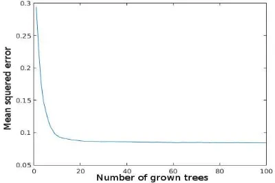
In order to build classifier, the data representing all training fields were used simultaneously. From each training data set 100 000 points representing both road and no-road classes were taken randomly. In the first pass 100 trees were grown utilising all components of the feature vector. This number of trees is sufficient to stabilise the mean squared error of generalisation (Figure 4).
Figure 4. Mean squared error as a function of the grown tree number
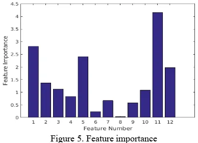
As a result of the first pass calculation, the variable importance of the particular features (Figure 5) and the generalisation error of 7% were estimated. The plot (Figure 5) shows the increase in mean squared error averaged over all trees and divided by their standard deviations, calculated for each variable separately.
Figure 5. Feature importance
Based on the results of the classifier training, the vector of the features was reduced. Due to low value of the importance of the 8th variable, the mean value of the deviation angles within 3 meter radius was removed from the feature vector. For the reduced vector of the features we received the generalization error of 7%. Therefore, the reduced set of features is as well effective as the original vector of features. The classifier built in the second pass was used in the further investigations.
All data representing the test fields were classified using constructed classifier. The level of certainty was set up on 85 %. It means that a point was classified as the road point if 85% of the trees voted for that. The results of classification were compared with the results of the manual classification. This comparison is given as the confusion matrix for the particular training field (Table 1, 2, 3) and for the evaluation field (Table 4).
manual Non-roads Roads Total
classification automatic classification
Non-roads 4 437 284 245 349 4 682 633
Roads 84 668 184 736 2 69 404
4 521 952 430 085 4 952 037
Table 1. Confusion matrix for the field 1
manual Non-roads Roads Total
classification automatic classification
Non-roads 4 615 897 89 103 4 705 000
Roads 125 355 156 293 281 648
4 741 252 245 396 4 986 648
Table 2. Confusion matrix for the field 2
manual Non-roads Roads Total
classification automatic classification
Non-roads 4 648 007 54 987 4 702 994
Roads 1 917 6 334 8 251
4 649 924 61 321 4 711 245
Table 3. Confusion matrix for the field 3
manual Non-roads Roads Total
classification automatic classification
Non-roads 4 736 704 502 377 5 239 081
Roads 47 041 344 632 391 673
4783745 847009 5 630 754
Table 4. Confusion matrix for the field 4
The values on the diagonal of the matrix represent values of the correct classification. The off-diagonal values are the numbers of points that were classified incorrectly (e.g. Table 1, values 245349 and 84668).
Moreover, for the accuracy assessment, the following parameters were estimated:
ICP – Overall classification accuracy
Kappa – kappa coefficient, overall classification agreement Ec1– Error of commission for class non-roads
Ec2 – Error of commission for class roads Eo1– Error of omission for class non-roads Eo2– Error of omission for class roads Ap1– producer's accuracy for class non-roads Ap2 – producer's accuracy for class roads Au1 – user's accuracy for class non-roads Au2 – user's accuracy for class roads
These values for the particular test fields are given in Table 6. Since the datasets of the test fields 1, 2 and 3 were used simultaneously for the classifier construction, the values given in the columns 2, 3 and 4 of Table 6 reflect the internal quality of the classifier. The values collected in the column 5 (Field 4) show the classification accuracy on the evaluation dataset, which can be interpreted as the absolute accuracy.
Parameter Field 1 Field 2 Field 3 Field 4
ICP 0.93 0.96 0.99 0,90
Kappa 0.92 0.95 0.99 0,87
Ec1 0.05 0.02 0.01 0,10
Ec2 0.31 0.45 0.23 0,12
Eo1 0.02 0.03 0.01 0,01
Eo2 0.57 0.36 0.90 0,59
Ap1 0.95 0.98 0.99 0,90
Ap2 0.69 0.55 0.77 0,88
Au1 0.98 0.97 0.99 0,99
Au2 0.43 0.64 0.10 0,41
Table 6. Accuracy ratings for trainingand evaluation fields
3.5 Road axes detection
As a result of the classification the point cloud is divided into two subsets: road points and non-road points. Since the level of certainty was set up at 85 % all points below this value have been classified as non-road points. The subset “road points” have been then converted to raster with 0.5 m pixel size. In order to achieve road axes, a set of binary morphological operations, implemented in Matlab, is utilised in the following order: majority, clean, thin, clean, diag.
4. RESULTS
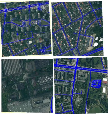
After the classification of the whole test area, the filtered point cloud representing roads was obtained. The resulting dataset contains only those points from source dataset that were assigned to class roads with 85% level of certainty. The classified points with the assigned level of certainty are shown in Figure 6 for a representative part of the study area.
Figure 6. Classification results (a part of the study area)
Some gaps are present in the data set representing road. These gaps are produced by cars and road overpasses. Unfortunately, overpasses were not present in the training datasets.
The detailed analysis of the results shown that involving the RGB in the vector of features improves the classification in the case of the presence of vegetation in the direct neighbourhood of the road.
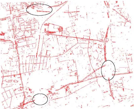
After the generation of the binary image and applying the morphological algorithms, the road axes were produced. The morphological operations were able to reduce small gaps (Figure 7). Nevertheless, the big gaps caused by overpasses still remain (ellipses in the Figure 7). Besides this issue, the overall accuracy and quality of the road detection is satisfactory.
Figure 7. Produced road axes (a part of the study area)
5. CONCLUSION
In this study, the random forests were successfully applied to detect the urban road in the ALS point cloud. ALS and imagery based parameters were selected as the components of the feature vector. After the feature evaluation by random forests, the local variation of the mean value of the normal vector (feature No 8) has been removed due to low importance. The most relevant features are intensity, number of echoes and height differences. The RGB features improve the classification in the presence of vegetation. We received the overall classification accuracy of 93%, 96 and 99% for three training datasets, respectively. For the evaluation dataset we received the overall accuracy of 90%.
The proposed approach at the current stage was not able to recognize correctly road overpasses. This issue should be addressed in the future work.
REFERENCES
Breiman, L., 2001. Random Forests. Mach. Learning 45, pp. 5– 32.
Breiman, L., Friedman, J., Olshen, R. and Stone, C., 1984. Classification and regression trees. Chapman & Hall, New York.
Chehata, N., Guo, L., Mallet, C., 2009. Airborne Lidar feature selection for urban classification using Random Forests. International Archives of Photogrammetry, Remote Sensing and Spatial Information Sciences. Vol. XXXVIII, Part 3/W8 – Paris, France, XXXVIII(c), pp. 207–212.
Choi, Y.W., Jang, Y.W., Lee, H.J., Cho, G.S., 2008. Three-dimensional LiDAR data classifying to extract road point in urban area. IEEE Geosci. Remote Sens. Lett. 5, pp. 725–729.
Clode, S., Kootsookos, P., Rottensteiner, F., 2004. The automatic extraction of roads from lidar data. Realt. Imaging 35, pp. 231–237
Ferraza, A., Mallet, C., Chehata,N., 2016. Large-scale road detection in forested mountainous areas using airborne topographic lidar data. ISPRSJournal of Photogrammetry and Remote Sensing. 112, pp. 23–36
Hu, X., Tao, C.V., Hu, Y., 2004. Automatic road extraction from dense urban area by integrated processing of high resolution imagery and Lidar data. International Archives of Photogrammetry, Remote Sensing and Spatial Information Sciences XXXV-B3, Vol. 35 (Part B3) (2004), pp. 288-292
Niemeyer, J., Rottensteiner, F., Soergel, U., 2013. Classification of urban LiDAR data using conditional random field and random forests. Proc. JURSE 2013 856, pp. 139 – 142
Shackelford, A.K., Davis, C.H., 2003. Fully automated road network extraction from high-resolution satellite multispectral imagery. IGARSS 2003. 2003 IEEE Int. Geosci. Remote Sens. Symp. Proc. (IEEE Cat. No.03CH37477) 1, pp. 461–463.