MULTITEMPORAL QUALITY ASSESSMENT OF GRASSLAND AND CROPLAND
OBJECTS OF A TOPOGRAPHIC DATASET
P. Helmholz a, b,1, T. Büschenfeldc, U. Breitkopf a, S. Müller a, F. Rottensteiner a
a
IPI – Institute für Photogrammetrie und GeoInformation, Leibniz Universität Hannover,
Nienburger Str. 1, 30167 Hannover, Germany; (helmholz, breitkopf, mueller, rottensteiner)@ipi.uni-hannover.de, b
Department of Spatial Sciences, Curtin University of Technology, GPO Box U1987, Perth WA 6845, Australia; [email protected] c
TNT - Institut für Informationsverarbeitung, Leibniz Universität Hannover, Appelstr. 9a, 30167 Hannover, Germany; [email protected]
Commission VI, WG VI/2
KEY WORDS: Automation, Quality, Inspection, Updating, GIS, Crop, Multitemporal, Classification
ABSTRACT:
As a consequence of the wide-spread application of digital geo-data in geographic information systems (GIS), quality control has become increasingly important to enhance the usefulness of the data. For economic reasons a high degree of automation is required for the quality control process. This goal can be achieved by automatic image analysis techniques. An example of how this can be achieved in the context of quality assessment of cropland and grassland GIS objects is given in this paper. The quality assessment of these objects of a topographic dataset is carried out based on multi-temporal information. The multi-temporal approach combines the channels of all available images as a multilayer image and applies a pixel-based SVM-classification. In this way multispectral as well as multi-temporal information is processed in parallel. The features used for the classification consist of spectral, textural (Haralick features) and structural (features derived from a semi-variogram) features. After the SVM-classification, the pixel-based result is mapped to the GIS-objects. Finally, a simple ruled-based approach is used in order to verify the objects of a GIS database. The approach was tested using a multi-temporal data set consisting of one 5-channel RapidEye image (GSD 5m) and two 3-channel Disaster Monitoring Constellation (DMC) images (GSD 32m). All images were taken within one year. The results show that by using our approach, quality control of GIS- cropland and grassland objects is possible and the human operator saves time using our approach compared to a completely manual quality assessment.
1
Corresponding author
1. INTRODUCTION
Today, many public and private decisions rely on geospatial information. Geospatial data are stored and managed in geographic information systems (GIS). In order for a GIS to be generally accepted, the underlying data need to be consistent and up-to-date. As a consequence, quality control has become increasingly important. A high degree of automation is required in order to make quality control efficient enough for practical application. This goal can be achieved by automatic image analysis techniques.
The basic methodology to represent the real world in a GIS is to define objects using a data model (e.g. a feature type catalogue also called GIS-object catalogue) which defines the objects to be contained, as well as their properties and structure. In the European Norm (DIN EN ISO 8402, 1995), quality is defined as the “Degree to which a set of inherent characteristics fulfils requirements”. In the context of GIS this means that, first, the data model must represent the real world with sufficient detail and without any contradictions (quality of the model). Second, the data must conform to the model specification (quality of the data). There are five important measures for the quality of geo-data: logical consistency, completeness, positional accuracy, temporal accuracy and thematic accuracy (EN ISO 9000:2005, 1995). Only the consistency can be checked without any comparison of the data to the real world. The other quality measures can be derived by comparing the GIS data to the real world as it is represented in satellite images. We call this step verification or quality assessment (Gerke and Heipke, 2008).
After reviewing related work in section 2, we will present our method for the quality assessment of cropland and grassland of a GIS data set with respect to the thematic accuracy. The
thematic accuracy is the percentage of correct objects in the GIS-database. In our approach we verify GIS cropland and grassland objects automatically comparing them with the real world in the form of remotely sensed images. Input data into the system are up-to-date multi-temporal satellite images taken in one year and a GIS which has to be verified. The system verifies the GIS-objects using automatic image analysis approaches introduced in section 3. The result of the automatic comparison of the GIS-objects and the images is the decision whether an object in the GIS data set is correct (accepted from the system; labelled green) or incorrect (rejected from the system; labelled red). The results of the automatic procedures are passed on to a human operator. All the accepted objects do not have to be reviewed, while for all rejected objects an interactive check by the human operator is necessary. The human operator saves time using our system for quality assessment because an interactive check of all GIS-object accepted by the system is not necessary anymore. We call this efficiency time efficiency. Because the final decision of rejected GIS-objects is done by the human operator, our approach is a semi-automatic one. However, given the fact that quality assessment is essentially carried out to remove errors in the GIS data base, classification errors from analysing the satellite images have to be avoided because these errors can lead to undetected errors remaining in the GIS database. The main goal of our approach is to achieve a certain thematic accuracy of the GIS database after the verification process.To evaluate our approach and to prove that
the approach is suitable for quality assessment, an evaluation is done in section 4. The paper concludes with a summary and an outlook in section five.
2. RELATED WORK
The focus of this paper is the verification of GIS-cropland and grassland objects. The publications dealing with the classes cropland and grassland using multi-temporal images are limited to the classification task. Therefore, in this section we will focus on approaches dealing with the classification of cropland, grassland and similar classes like vineyards using a multi-temporal data set with low resolution images. The special focus will be on features and on the classification method.
Using a multi-temporal data set with low resolution images, it is common to use only spectral features for the classification process (Gong et al., 2003; Itzerott and Kaden, 2007; Marçal und Cunha, 2007; Hall et al., 2008). Itzerott and Kaden (2007) use for the classification of different agricultural classes norm-curves of these classes which were created from a prior multi-temporal analysis based on the Normalised Difference Vegetation Index (NDVI). These NDVI-norm-curves show that grassland objects always have an NDVI significantly larger than zero, whereas cropland can have a very low NDVI depending on the season. The norm-curves are created using four Landsat images (GSD: 30m) taken within one year. For the classification of unknown GIS-objects of a given field boundary cadastre the mean NDVI of each object is calculated. Then a classification is carried out using the NDVI norm-curves within a Maximum-Likelihood or box classification. Using the box classification an overall accuracy of 65.7% and using the Maximum-Likelihood classification an overall accuracy of 72.8% could be achieved. However, the NDVI of different crops can underlie strong regional and temporal variations. Hence, the adaption of the NDVI-norm-curves to other regions is a challenge. Training with a multi-temporal data set within a large area would be necessary.
Simonneaux et al. (2008) apply a pixel-based approach using a decision tree algorithm for the classification of different kinds of crops. For each pixel a NDVI profile over time is calculated. To create these profiles, eight Landsat satellite images taken within one year were available. The overall accuracy of this approach is 83.7%; the kappa-index is 0.78. These good results could be achieved mainly through the high number of images.
Marçal and Cunha (2007) use the NDVI and a field boundary cadastre for the detection of vineyards in a multi-temporal data set consisting of nine SPOT 5 images (GSD: 5 m) taken in 2002, 2003 and 2005, and in addition four Chris Proba satellite images taken in 2006 (GSD: 17 m, 18 bands). Besides the average NDVI value also the minimum, maximum, standard deviation and the median NDVI per GIS-object was calculated. Marçal and Cunha (2007) summarise in their article that the features are useable for the classification but quantitative results are not presented.
Lucas et al. (2007) proposes a rule based classification based on the software eCognition (Baatz and Schape, 2000). First, segments (fields) are determined by a segmentation of each GIS-object. Next, numerical decision rules based on fuzzy logic are developed to discriminate vegetation classes. The rules are primarily based on inferred differences in phenology, structure, wetness and productivity. The decision rules connect knowledge about ecology and the information content of single and multi-temperal remotely sensed data and their derived products (e.g., vegetation indices). The rule-based classification
gives a good representation of the spectral and temporal characteristics of different agricultural classes but leads to quite complex rules. These complex rules are difficult to manage and the transfer to other regions.
De Wit and Clevers (2004) apply a pixel-based Maximum-Likelihood classification combined with an object-based decision tree classification. In the pixel- and object-based classification the NDVI was used as feature. The image data set used in (De Wit and Clevers, 2004) consist of in total 13 Landsat, two IRS-LISS3 (GSD: 25 m) and two ERS2-SAR images taken within two years. The overall accuracy of this approach is high with 90.4%. However, for the object-based classification first the interactive creation of a field boundary by a human operator is necessary. Due to the time-consuming generation of the field boundary cadastre, further improvement for a practical use of this approach is necessary.
If images of higher resolution are available, additional features like textural or structural features can be introduced into the classification process. Textural features describe the distribution of grey values; structural features describe structures within a GIS-object such as parallel lines within a local neighbourhood of a pixel or within a GIS-object. For instance, Müller et al. (2010) use spectral, textural and structural features in a classification based on weighting functions to differentiate between several kinds of crops. They use high resolution multi-temporal aerial images (GSD: 17cm). First, the phenological behaviour of different crops is trained using a training data set and the determined features. Based on this training, GIS-objects with an unknown class can be classified by analysing their phenological behaviour. The results are promising with an overall correct classification rate of 91.3% but due to the small size of the test area no final conclusions about the practical usefulness can be made.
Our method differs from the cited approaches by the used features, classification method and number of images needed for the classification/verification. For instance, we use structural features derived from a semi-variogram. For classification we use is the state-of-the-art algorithm of Support Vector Machines (SVM; Vapnik, 1998) which has not been used for the multi-temporal classification of the agricultural classes cropland and grassland so far. In addition, to avoid the use of a field boundary cadastre, we apply a pixel-based classification. Our approach is flexible regarding to the number of images, and also can operate with only three images taken in one year.
3. APPROACH
The idea of the approach is to use the fact that the appearance of cropland changes significantly within a year (cropland can be covered with vegetation or is not covered with vegetation, it can contain structures when tilled or not when untilled, ...) whereas the difference in the appearance of grassland changes only slightly. As mentioned above, these multi-temporal characteristics are considered in a pixel-based classification approach. In order to process the classification three main steps are necessary. First, features are extracted within a local Nf x Nf
neighbourhood. Second, these features are classified by a previously trained supervised learning method. Finally, the pixel-based results are transferred to the GIS-objects. The object boundary polygons are given by the GIS data set which has to be verified.
3.1 Feature Extraction
The feature extraction process takes into account several different aspects to ensure an optimal classification result. For
the classification spectral, textural and structural features are used.
3.1.1. Feature extraction Information about vegetation is contained in the bands of multispectral images and in features derived from them (Ruiz et al., 2004; Hall et al., 2008; Itzerott and Kaden, 2007). Similar to the cited works, we use the median value of a local neighbourhood of each channel for the classification. Furthermore, the variance is used as an additional feature in the classification process. The dimension Nspec of the
feature vector for the spectral features xspec per band is two.
Textural features derived from of the grey level co-occurrence matrix (GLCM)) can give important hints to separate different agricultural classes (Haralick et al., 1973; Rengers und Prinz, 2009). We use eight Haralick features energy, entropy, correlation, difference moment, inertia (contrast), cluster shade, cluster prominence, and Haralick correlation (Haralick et al., 1973) in our classification approach. Using three directions, the dimension Ntex of the feature for the textural features xtex is 24
per band.
In addition, structural features can give an important hint for the classification of the agricultural classes cropland and grassland (Helmholz, 2010), whereas the usefulness of these features mainly depends on the resolution of the available images. While parallel straight lines caused by agricultural machines are visible in cropland GIS-objects in images with a higher resolution, these lines vanish in images with a lower resolution. However, because these structures can give an important hint in order to separate cropland and grassland and because our algorithm should have the possibility to be easily applied to other image data (such as high resolution images), we use structural features. The structural features are derived from a semi-variogram. Features derived from a semi-variogram have been successfully used for the classification of different agricultural areas in (Balaguer et al., 2010). In total 14 features (Balaguer et al., 2010) are used in the classification process. The dimension Nstruc of the feature vector of the structural
features xstruc per band is 14.
3.1.2. Feature vector The feature vector of a pixel xfeat per
band is build by concatenation of the feature vectors with
xT
feat = (xTspec, xTtex, xTstruc) (1)
the dimension Nfeat is
Nfeat = Nspec + Ntex + Nstruc = 40 (2)
To maintain flexibility with respect to various image acquisition systems and sensors, respectively, an arbitrary number of input channels Nch is supported. All input channels are sub-sampled
equally by a factor leading to an image pyramid for every channel, whereas Nres is the number of pyramid levels. Each
pyramid level is handled equally. The set is passed on to the feature extraction module, where spectral, textural and structural features are calculated for each pixel within an Nf x Nf
neighbourhood as described before. Features extracted at the same pixel position build up one feature vector xfeat_total.
The dimension dfeat_total of the feature vector xfeat_total is:
dfeat_total = Nch · Nres · Nfeat (3)
For instance, using multispectral and multi-temporal information of one five band image and two three-band images simultaneously, the number of bands is Nch = 11. Assuming Nres
= 2 resolution levels, we get 22 bands for which a feature vector with Nfeat = 40 has to be calculated. Thus, the dimension of the
feature vector is dfeat_total = 880.
3.2 Pixel-based Classification
The classification is carried out using SVM. The SVM classifier is a supervised learning method used for classification and regression. Given a set of training examples, each marked as belonging to one of two classes, SVM training builds a model that predicts whether a new example falls into one class or the other. The two classes are separated by a hyperplane in feature space so that the distance of the nearest training sample from the hyperplane is maximised; hence, SVM belong to the class of
max-margin classifiers (Vapnik, 1998). Since most classes are not linearly separable in feature space, a feature space mapping is applied: the original feature space is mapped into another space of higher dimension so that in the transformed feature space, the classes become linearly separable. Both training and classification basically require the computation of inner products of the form ΦΦΦΦ(xi)T⋅ΦΦΦΦ(xj), where xi and xj are feature vectors of two samples in the original feature space and ΦΦΦΦ(xi) and ΦΦΦΦ(xj) are the transformed features. These inner products can be replaced by a Kernel function K(xi,xj), which means that the
actual feature space mapping ΦΦΦΦ is never explicitly applied
(Kernel Trick). In our application we use the Gaussian Kernel
K(xi, xj) = exp(-γ⋅ || xi – xj||2). The concept of SVM has been
expanded to allow for outliers in the training data to avoid over-fitting. This requires a parameter ν that corresponds to the fraction of training points considered to be outliers. Furthermore, classical SVM only can separate two classes, and SVM do not scale well to a multi-class problem. A common way to tackle this problem is the one-versus-one-strategy (Chang and Lin, 2001) where all combinations of classes C are tested against each other. In total C(C-1)/2 combinations are calculated. The pixel is assigned to the class with the most wins (winner-takes-it-all-strategy).
For our approach, the SVM algorithm needs to learn the properties of the different classes. These are not only the classes cropland and grassland but classes which describe a typical site, e.g. settlement, industrial area and forest. The training is done using a set of image patches with known class labels. The image patches and the class labels are assigned to the training objects interactively by a human operator. Each feature is normalised so that its value is between 0 and 1. Then, all feature vectors are used to train the SVM classifier required for the one-versus-one
strategy. The result of the classification process is a labeled map, which represents the class membership for each pixel.
3.3 Transfer the pixel-based classification results to GIS-objects
After the pixel-based classification was utilised, the result for all pixels inside an object must be transferred to a GIS-object. This is done using the approach from Busch et al. (2004). Pixels that match the class of the GIS object are considered as correct, while pixels belonging to another class are considered to be
incorrect. Two criteria are chosen for the assessment of the GIS objects. First, the ratio q of incorrect pixels in relation to all pixels that cover the object are calculated using
q = incorrect / (correct + incorrect) (4)
If q is larger than the pre-defined threshold tq, the GIS object
will be labelled as rejected/incorrect. The threshold tq depends
on how many incorrect pixels are likely to appear in a cropland or grassland object.
As incorrect pixels can be distributed more or less equally in the object due to noise or inhomogeneously textured regions, a second criteria considering the compactness of an error region
is necessary. A compact error is an area of connected pixels belonging to the same class (which differs from the class label in the GIS data set) with a width larger than a threshold tw and
an area larger than a threshold tA. The width of an assumed
compact error is determined applying a morphologic filter (erosion) and counting the steps till the assumed compact error disappears. A GIS object with a compact error is labelled as rejected/incorrect and has to be reviewed by a human operator.
4. EVALUATION 4.1 Data
To evaluate our approach we have used the European CORINE Land Cover GIS database (CLC) and three multi-temporal images taken in one year covering a test site of 329 km2 in Halberstadt, Germany. For the evaluation, a reference dataset was available. The reference dataset was produced using visual interpretation of the images.
4.1.1. Image Data Images are available from two different sensors, namely RapidEye and DMC (Disaster Monitoring Constellation, operated by DMC International Imaging (DMCii)). The images were acquired within a 4 month period during the summer months. The RapidEye image was acquired on August 20, 2009 and has a resolution of 5m. The five bands of this sensor are blue, green, red, red edge and near infrared. In addition two DMC images are used, acquired on April-24, 2009 and on August-24, 2009. The DMC sensor has a resolution of 32m and captures three bands (green, red and near infrared). The dimension of Nch is 11 (5 + 2x3). For textural information,
the resolution was subsampled by a factor of two to cover relevant information. Hence, the resulting dimension of the feature vector for one pixel position is 440. The neighbourhood is Nf = 11 pixels for all scenes to cover a relevant area. All
images are orthorectified.
Before processing all images in one workflow the 32m DMC images are clipped to the same size and resampled to the same resolution as the RapidEye image. For the resampling we use a nearest neighbor interpolation, because radiometric information remains unaltered (Albertz, 2001).
4.1.2. GIS database The European CLC data set is managed and coordinated by the European Environment Agency (EEA, 2011), assisted by the European Topic Center for Land Use and Spatial Information (ETC-LUSI). In Germany the UBA (Umweltbundesamt – Federal Environmental Agency) is the national reference center. It acts as the contact point for the EEA and is responsible for the management and coordination of CLC. The data model was defined to be compliant with a scale of 1:100,000; the minimum mapping unit is 25 ha for new polygons and 5 ha for changes of existing polygons. The CLC data set has been produced with respect to reference years 1990, 2000 and 2006 using mainly images of Landsat, SPOT and IRS satellites. Even though the minimum mapping unit is 25 ha, GIS-objects with an area smaller than 25 ha appear in the data set of our test site. GIS-objects smaller than 1 ha were not processed with our approach, because a reliable classification of small GIS-objects using DMC images with a resolution of 32 m is not possible.
The main land cover class in our test site is cropland. Out of 425 km2 with 3072 GIS cropland and grassland objects, 1316 cropland GIS-objects covering 367 km2 with an average size of 27.9 ha, and 1756 grassland GIS-objects covering 58 km2 with an average size of 3.3 ha can be found.
4.2 Evaluation assessment
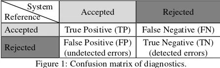
Confusion matrices are a common tool for quality assessment. For the verification a special confusion matrix is used which compares the verification result (accepted/rejected GIS-objects) with a reference (correct/false GIS-objects). Such a confusion matrix is visualised in Figure 1.
System
Reference Accepted Rejected
Accepted True Positive (TP) False Negative (FN)
Rejected False Positive (FP) (undetected errors)
True Negative (TN) (detected errors) Figure 1: Confusion matrix of diagnostics.
Based on this confusion matrix, measures for the evaluation can be derived, e.g. the thematic accuracy. The goal is to increase the thematic accuracy. The thematic accuracy before the verification process is TA a priori with
TA a priori = (TP + FN)/(TP + FN + FP + TN) x 100% (4)
The aim is to achieve a thematic accuracy after the verification process TA a posteriori with
TA a posteriori = TA a priori + TN/(TP + FN + FP + TN) x
100% (5)
whereas TA a posteriori has to be at least 95%. At the same time the human operator should save time compared to a completely manual quality assessment of the GIS data set. A measure which represents this goal is the time efficiency with
time efficiency =(TP + FP)/(TP + FN + FP + TN) x 100% (6)
which is equal to the percentage of GIS-objects which do not have to be reviewed by a human operator. The time efficiency
should be at least 50%. The defined requirements are based on experiences gained from the practical application of quality assessment of GIS data sets (BKG, 2009).
4.3 Parameter settings
Only a small number of parameters have to be set to run our approach. Most of them can be trained automatically, others are defined by the characteristics of the used GIS and only a few of the parameters have to be set to empirical values.
The fact that the goal of our approach is the verification of a GIS data set influences the strategy of the classification process. The parameters of our method have to be optimised in order to achieve a good verification, but not necessarily a good classification result. For instance, a classification error which leads to an undetected error remaining in the GIS data set is penalised higher than classification errors which lead “only” to a false negative.
There are no parameters to be set for the calculation of the spectral features. Parameters for the feature extraction of the textural features are distance ∆ and direction α for the determination of the GLCM (Haralick et al., 1973). The parameters were set to the standard values ∆ = 1 and α = 0°, 45°, 90°, 135°. By using fixed parameters for∆ and α the textural features are only representative for these chosen parameters. By using four different directions for α the textural features are rotation invariant. Therefore, the dependency from the parameter α could be eliminated as far as possible. In contrast, the dependency from parameter ∆ could not been solved, so pattern which are not in the range of ∆ are not be taken into account.
For the semi-variogram feature extraction, three major parameters had to be set. As proposed in (Balaguer et al., 2010), we use six directions to calculate an omnidirectional semi-variogram. To obtain significant information about the occurring structures, a radius of 30 pixels with one pixel step size was chosen based on the RapidEye images (5m GSD).
There are further parameters for SVM classification. We decided to use the one-versus-one-strategy for the multi-class-SVM; the classes are cropland, grassland, settlement, industrial areas, deciduous and coniferous forest. In this paper we will focus only on the classes cropland and grassland. The parameter γ for the Gaussian Kernel as well as the parameter ν to avoid the over-fitting are learnt automatically using a cross validation with grid search (Hsu et al., 2010). The used training data are visualised in Figure 2.
Figure 2: GIS training objects (settlement (green), industrial areas (blue), cropland (turquoise), grassland (pink), deciduous
forest(yellow), coniferous forest (brown)).
To transfer the pixel-based classification results to GIS-objects there are three parameters. The threshold tq (see equation 4)
depends on how many incorrect pixels are likely to appear in a cropland or grassland object. For instance, a cropland area can be surrounded by shrubs or trees, so it is likely that pixels are classified as forest. tq can be set easily by an experienced human
operator. The parameters tA and tw are given by the definitions in
the GIS object catalogue. tw depends on the minimum mapping
areas of other classes than cropland/grassland and is set to 40 m; tA is given directly by the GIS object catalogue by the
minimum mapping areas of the classes others than cropland/grassland, e.g. ‘forest’, ‘settlement’ or ‘industry’. It is set to 1 ha.
Basically, the only parameters which have to be set by the human operator are ∆ (textural feature) and tq (to transfer the
pixel-based results to GIS-objects). In this publication we will focus on the setting of the parameter tq, as experience shows
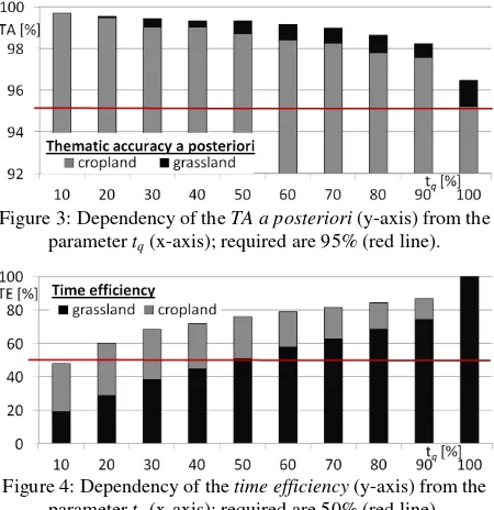
that this parameter has a high impact to the verification result. The parameter tq is tested using a series of variable values of tq
starting from tq =10% to tq =100%. The results of this analysis
are summarised regarding the TA a posteriori in Figure 3 and regarding the time efficiency in Figure 4. By setting tq to 10%
not more than 10% of incorrect pixels (equation 1) are allowed within a GIS-object. Therefore, the TA a posteriori is really high (nearly all errors can be detected) but the time efficiency is low (nearly all GIS-objects have to be reviewed by a human operator). If tq is increased, the setting is less strict. For tq =
100% the TA a posteriori decreased to the same level as the TA a priori (no errors could be detected; cropland 95.2%; grassland
96.5%) but at the same time the time efficiency is 100% (no manual effort for the human operator). Our aim is to find a setting which is strict enough to find errors in the GIS data set but not too strict, so the human operator can save time using the approach.
Figure 3: Dependency of the TA a posteriori (y-axis) from the parameter tq (x-axis); required are 95% (red line).
Figure 4: Dependency of the time efficiency (y-axis) from the parameter tq (x-axis); required are 50% (red line).
Because the required TA a posteriori of 95% could be achieved already before the verification process, the results regarding the
time efficiency is used to determine the best value for tq. For the
threshold tq = 60% the time efficiency achieves the required
50% for both classes (cropland and grassland) for the first time. Therefore, the parameter tq is set to 60% for the detailed
analysis in section 4.4.
4.4 Results
The evaluation results of our approach in form of confusion matrices are summarised in Figure 5 to Figure 7. In all cases the required thematic accuracy of 95% was already given (above 95%). However, the thematic accuracy could be increased to 98% to 99%, whereas the human operator has to review less than 50% of GIS-objects.
System
Reference Accepted Rejected
Accepted 65.5% (2012) 30.4% (935)
Rejected 1.2% (36) 2.9% (89)
Figure 5: Evaluation results of set union of the classes cropland and grassland (TA a priori = 95.9%, TA a posteriori = 98.8%,
time efficiency = 66.7%).
System
Reference Accepted Rejected
Accepted 77.2% (1016) 18.0% (237)
Rejected 1.6% (21) 3.2% (42)
Figure 6: Evaluation results of the class cropland (TA a priori = 95.2%, TA a posteriori = 98.4%, time efficiency = 78.8%).
System
Reference Accepted Rejected
Accepted 56.7% (996) 39.7% (698)
Rejected 0.9% (15) 2.7% (47)
Figure 7: Evaluation results of the class grassland (TA a priori = 96.5%, TA a posteriori = 99.1%, time efficiency = 57.6%).
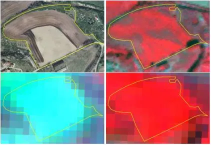
An example of a correctly rejected grassland GIS-object is given in Figure 8. While the GIS cropland object was covered with vegetation on the pictures on the right hand side, the picture in the second row on the left hand side does not show any vegetation. As grassland is covered by vegetation all year (Itzerott and Kaden, 2007), this GIS-object has to be grassland and not cropland as indicated in the GIS data set. This result can be confirmed by taken a look at the aerial image on the upper row on the left hand side. The aerial orthoimage is used to prove the result; it was not used within the verification process. The decision of our system to reject the GIS-object is correct.
Figure 8: Correct rejected grassland GIS object: aerial orthophoto, April 2009 (top left), RapidEye CIR - 27.09.2009 (top right) -
24.04.2009 (bottom left) - 24.08.2009 (bottom right).
5. CONCLUSIONS AND OUTLOOK
The method for the verification of cropland and grassland objects described in this paper achieved satisfactory for both classes even that the results from the class cropland are slightly better. In this publication we determined a suitable value for parameter tq. tq is important to transfer the classification result
to a GIS-object and has a big influence on the verification results. An investigation regarding the other parameters which needs experiences from a human operator to be set still has to be done.
Furthermore, a detailed analysis of the relevant features would be interesting, in order to reduce the feature vector to the most relevant features, and at the same time to reduce the necessary numbers of training areas. Maybe the best choice of features even could be determined during the training phase.
In addition, the approach was tested on only one multi-temporal multi-spectral data set so far. It is interesting to see the performance on further data sets. Especially because two out of the three images were taken to approximately the same time (only a few days different), the appearance of the vegetation hardly changes. Tests showed that using only the RapidEye images the results were comparable to using all three images; comparable means that the time efficiency was slightly lower and the TA a posteriori slightly higher.
In this paper we focused only on the classes cropland and grassland. The features should be useable to achieve also good results for further classes, e.g. the separation of different forest types (deciduous and coniferous forest).
ACKNOWLEDGEMENTS
This work was supported by the German Federal Agency for Cartography and Geodesy (BKG) in Frankfurt am Main.
REFERENCES
Albertz, J., 2001. Einführung in die Fernerkundung. Wissenschaftliche
Buchgesellschaft, Darmstadt, Germany.
Baatz M and Schape A (2000) Multiresolution segmentation-an optimization approach for high quality multiscaleimage segmentation. Angewandte Geographische Informationsverarbeitung XII. (Eds: Strobl, J. and Blaschke, T.), Beitrage zum AGIT- Symposium, Salzburg 2000, Karlsruhe, Herbert Wichmann Verlag, pp.12–23
Balaguer, A., Ruiz, L. A., Hermosilla, T., Recio, J.A., 2010. Definition of a comprehensive set of texture semivariogram features and their
evaluation for object-oriented image classification. Computers &
Geoscience, 36, pp. 231–240.
Busch, A., Gerke, M., Grünreich, D., Heipke, C., Liedtke, C. E., Müller,
S. 2004. Automated Verification of a Topographic Reference
Dataset: System Design and Practical Results. IntArchPhRS, vol. 35,
no. B2, pp. 735–740.
Chang, C.C. and Lin, C.J., 2001. LIBSVM: a library for support vector
machines. http://www.csie.ntu.edu.tw/˜cjlin/libsvm, accessed: 09/2010.
De Wit, A. J. W. and Clevers, J. G. P. W., 2004. Efficiency and accuracy of per-field classification for operational crop mapping. International Journal of Remote Sensing, 25(20), pp. 4091–4112.
DIN, EN, ISO (Hrsg.), Qualitätsmanagement. Begriffe. DIN EN ISO
8402: 1995-08. Berlin, 1995.
EEA - European Environment Agency, 2011: Corine Land Cover. http://www.eea.europa.eu/publications/COR0-landcover, (accessed: 06/2011).
Gerke, M. and Heipke, C., 2008. Image based quality assessment of
road databases. International Journal of Geoinformation Science (22),
No. 8, 2008, pp. 871–894.
Hall, A., Louis, J., Lamb, D., 2008. Low-resolution remotely sensed images of winegrape vineyards map spatial variability in planimetric
canopy area instead of leaf area index. Australian journal of grape and
wine research, vol. 14, no. 1, pp. 9–17.
Haralick, R.M., Shanmugam, K., Dinstein, 1973. Texture features for image classification. IEEE Trans. On Systems, man. And Cibernetics, SMC-3, pp. 610–622.
Helmholz, P., Rottensteiner, F., Heipke, C., 2010. Automatic qualtiy control of cropland and grassland GIS objects using IKONOS Satellite
Imagery. IntArchPhRS, vol. 38, no 7/B, pp. 275–280.
Itzerott, S. and Kaden, K., 2007. Klassifizierung landwirtschaftlicher
Fruchtarten. Photogrammetrie Fernerkundung Geoinformation (PFG),
vol. 2, 2007, pp. 109–120.
Lucas, R., Rowlands A., Brown A., Keyworth, S. and Bunting, P., 2007. Rule-based classification of multi-temporal satellite imagery for
habitat and agricultural land cover mapping. ISPRS Journal of
Photogrammetry & Remote Sensing, 62(3), pp.165–185.
Müller, S., Heipke, C. and Pakzad, K., 2010. Classification of farmland
using multitemporal aerial images. IntArchPhRS, vol. XXXVIII, part
4-8-2/W9, Haifa, pp. 70–74.
Rengers, N. and Prinz, T., 2009. JAVA-basierte Texturanalyse mittels Neighborhood Gray-Tone Differenz Matrix (NGTDM) zur Optimierung
von Landnutzungsklassifikation in hoch auflösenden
Fernerkundungsdaten. PFG, vol. 5, pp. 455–467.
Ruiz, L.A., Fernàndez-Sarrìa, A. and Recio, J.A., 2004. Texture
feature extraction for classification of remote sensing data using
wavelet decomposition: A comparative study. IntArchPhRS, vol.
XXXV, pp. 1109–1115.
Simonneaux, V., Duchemin, B. , Helson, D. , Er-Raki, S. , Olioso, A. and Chehbouni, A. G., 2008. The use of high-resolution image time series for crop classification and evapotranspiration estimate over an
irrigated area in central Morocco. International Journal of Remote
Sensing, 29(1), pp. 95–116.
Vapnik, V.N., 1998 Statistical Learning Theory. Wiley, New York,
USA.