Response of spray drift from aerial applications at a forest
edge to atmospheric stability
David R. Miller
∗, Thomas E. Stoughton
Department of Natural Resources Management and Engineering, The University of Connecticut, Storrs, CT 06269-4087, USA
Received 22 February 1999; accepted 5 August 1999
Abstract
A biological pesticide was aerially applied to a hardwood forest – corn field edge in a replicated series of single spray swaths. The drift of small droplets, which remained suspended in the air after each spray swath, was monitored remotely and mapped with the University of Connecticut portable, elastic-backscatter lidar. Plumes of small droplets were tracked which drifted off after every spray swath and dispersed into the atmospheric boundary layer.
Plume movement and the rate of near field plume dilution was primarily dependent on the stability of the atmosphere, which implies that concentrations in the air in adjacent areas can be partially controlled by correct timing of the spray operations. The study results support the hypothesis that widespread dispersal of a small amount of pesticide is inevitable, even in well-conducted spraying operations. ©2000 Elsevier Science B.V. All rights reserved.
Keywords:Spray drift; Lidar; Forest edge; Atmospheric stability; Pesticide; Application
1. Introduction
Trace amounts of pesticides and their degradation products (Somasundurama and Coats, 1991) can be found worldwide (Kurtz, 1962; Majewski and Capel, 1995). The chances of this causing increases in pest resistance, ecosystem damage and harmful effects on humans has not been quantified but has been suspected since the Silent Spring of Carson (1962). There are no specific guidelines on control of the fraction of spray that disperses into the atmosphere during ap-plication operations because it has never been
defini-∗Corresponding author. Tel.:+1-860-486-2840;
fax:+1-860-486-5408.
E-mail address:[email protected] (D.R. Miller).
tively demonstrated or quantified in spray application experiments.
The US Environmental Protection Agency (EPA) defines drift as the movement of a pesticide through the air off the target site during or immediately after application or use (Holst and Ellwnager, 1984). Off the target site can mean deposited in immediately ad-jacent areas or ‘extended airborne displacement’. The majority of the extensive research and trade literature on the topic is aimed at technology and techniques to control the drift immediately downwind from spray operations. Bache and Johnstone (1992) and Picot and Kristmanson (1997) provide recent reviews.
A general consensus exists in the applicator com-munities that spray remaining in the atmosphere is a very small and inconsequential proportion of the pes-ticide material applied. For example, the recent
maries of studies by the corporate Spray Drift Task Force (1997) do not mention spray escaping into the atmosphere. Modern spray application computer mod-els, such as FSCBG (Teske et al., 1992) developed by the USDA Forest Service and AGDRIFT (Hewitt et al., 1997) from the pesticide industry Spray Drift Task Force, which are recommended to guide operations, simulate ensemble average deposition out to several hundred meters from the spray site. They do not, how-ever, calculate spray droplets drifting upward into the atmosphere. Several random walk Lagrangian models have been reported (Walklate, 1992; Wang et al., 1995; Picot and Kristmanson, 1997; Aylor, 1998) which do calculate a fraction of material remaining in the air. Only one of these, the PKBW model of Picot and Kristmanson (1997), is available for general applica-tion. None of the estimations of spray moving upward from the spray sites has been field verified. Thus a specific connection between common agriculture, hor-ticulture and forest spray applications and widespread trace occurrence in the environment has not generally been made.
We have recently demonstrated, with remote sens-ing lidar (light detection and rangsens-ing) measurements of aerial spray over forests, that a plume of small drops remains suspended in the air and is dispersed through the atmospheric boundary layer in the same manner as other air pollutants (Stoughton et al., 1997). Once dispersed over distances of tens to hundreds of kilometers, this material and its degradation products can only be removed from the atmosphere by rain-fall and turbulent diffusion deposition mechanisms. The purpose of this paper is to present replicated li-dar measurements (visualizations) of aerially applied spray dispersing over a forest into the atmospheric boundary layer. It also presents the relationships of the plume movement to varying atmospheric conditions.
2. Methods
The study was conducted on 4–6 September 1997 on the University of Connecticut Forest and adjacent re-search farm in Coventry, Connecticut at 41◦47′30′′N,
72◦22′29′′W. The site was a 4 ha cornfield adjacent to
a hardwood forest edge. The edge was oriented in a N–S direction, with a S to N bearing of 15◦. The
for-est was 20 m tall and a 35 m tall micrometeorology tower was located 200 m inside the forest edge. A fast response, sonic anemometer (Gill Inst. Ltd., Solent Research ultrasonic anemometer) measured the three components of the wind (u,v, w), and the tempera-ture at 10 m above the forest canopy at 0.1 s intervals. Humidity was measured at 1 min intervals with a slow response, aspirated electronic hygrometer (Campbell Scientific, CS500) at the same level.
A Cessna Ag-Truck spray airplane equipped with 8003 flat fan nozzles sprayed a solution of 5% wa-ter with ‘gypchek’, a nucleopolyhedrosis virus used as a biological pesticide for Gypsy Moth (Lymantria disparL.). The remaining solution was 2% bond and 93% carrier 038 (Abbot Labs). The carrier was 51% water resulting in an overall water fraction (volatile fraction) of 52%. The spray was applied at a rate of 9.35 l ha−1. The initial drop size, volume mean
diam-eter (VMD) from the nozzles was ∼175m (Richard
Reardon, USDA Forest Service, personal communi-cation). The spray was applied in single 400 m long swaths parallel to the forest edge. In swaths where the wind direction was into the edge the swath was flown 40 m outside the edge. When the wind was out of the edge, the swath was flown 40 m inside the forest. The spray height was 10 m (±5 m) above the forest canopy. The University of Connecticut elastic backscatter li-dar, described in detail by Stoughton et al. (1997), was used to track the drifting spray plumes. The lidar is a laser remote sensing system which, similar to radar, can scan through a plume of spray droplets in horizon-tal and vertical slices. It measures the laser light inten-sity backscattered from the aerosols suspended in the air. The backscatter intensity is a function of the con-centration of droplets in the air, the particle size distri-bution, the composition (refractive index) and shape of the aerosols. In this study we interpret differences in relative backscatter to be primarily due to differences in droplet number concentration.
op-Fig. 1. Location map of the experimental site.
Table 1
Hardware configuration of the lidar during the spray runs
Wavelength (mm) 1.064
Energy per pulse (mJ) 125
Repetition rate (Hz) 50
Pulse width (ns) <15
Pulse to pulse stability ±3%
Detector type Avalanche photodiode High quantum efficiency 40%
Useful area (mm2) 7
erational parameters and scan sequences used during the spray runs. Fig. 1 is a map of the site showing the locations of the spray swaths, lidar, and micrometeo-rology tower.
3. Results
After each spray swath, most of the material sprayed was contained in droplets larger than 100m which
Table 2
Lidar scan sequences and operational parameters during the spray runs
Run Scan type Elevation range (◦) Azimuth range (◦) Step size (◦) Number of scans
1 Horizontal – 35 0.5 3
Vertical 9 – 0.5 48
2, 3, 4 Horizontal – 35 0.5 5
Vertical 9 – 0.5 80
deposited on the foliage and ground below where cov-erage was complete. In each case, however, plumes of spray droplets containing an unquantified amount of material, remained suspended in the air and dispersed into the atmosphere. The period of time that it took to disperse was primarily dependent on the stability of the atmosphere. The mean wind controlled the direc-tion and speed of plume translocadirec-tion away from the target site.
Four swaths are shown, in Figs. 2, 3, 4 and 5, of nine available in the three day experiment. The four represent the wide variation in stability and wind con-ditions encountered when aerial spraying is commonly conducted from stable, calm conditions to unstable, windy conditions. The remaining 5 swaths were within the range of atmospheric conditions represented by the four examples. Table 3 lists the atmospheric con-ditions during the run periods. Data are presented for each spray swath as sequential two-dimensional maps showing contours of equal lidar backscatter in a sin-gle vertical slice through the plume. The sequences start 1 min after the spray plane passed which was enough time for all of the large drops to fall out onto the vegetation surfaces below and immediately down-wind. Therefore, only the smaller suspended droplets remained in the air. The aerosol clouds shown in the lidar scans could not be seen by eye. Corresponding descriptions of the plume movement and dispersion are presented in the paragraphs below listed by swath number and corresponding figure.
3.1. Swath 1 (Fig. 2)
Fig. 2. Vertical cross plume scans through the Run 1 plume showing the evolution of the plume at a single location. Each contour map shows thex,zspatial distribution of backscatter intensity indicating relative droplet density. The plume is shown at 1 min intervals after the single pass of the spray plane.
350 m. It had dispersed vertically to about 170 m above ground. During the second minute after spraying the plume continued to move at about 4 m s−1and contin-ued to break up and dissipate. After three minutes the plume had dispersed enough that it could no longer be detected with the lidar.
3.2. Swath 2 (Fig. 3)
This swath was made under unstable conditions and wind speeds similar to swath 1, but in the afternoon rather than the early morning. In this case the ver-tical spread of the plume is most striking with the
plume spreading vertically over 175 m after 2 min and the highest concentrations are elevated well above the release height. The plume remained about 100 m in width, throughout. The plume did not break up and dissipate as fast as those during the earlier higher wind conditions. The organized plume could still be de-tected after 3 min but not after 4 min.
3.3. Swath 3 (Fig. 4)
Fig. 3. As Fig. 2 for Run 2.
calm/unstable to calm/stable conditions. The air-craft sprayed the swath outside the forest edge and the plume did not move. In fact, it remained near the ground and spread slowly. Therefore, it was easily detected a full 5 min after spray-ing. There was no plume rise due to the stable conditions.
3.4. Swath 4 (Fig. 5)
This early morning swath was made in stable, calm conditions. The plane sprayed the swath over the canopy and the plume drifted out of the edge at a speed of about 0.4 m s−1. Over the 5 min shown, the
Fig. 4. As Fig. 2 for Run 3.
100 m in width, extended vertically to 120 m above the ground and moved several hundred meters downwind. The decay of lidar backscatter from the plume with time in nine swaths, two during stable atmospheric conditions and seven during unstable conditions, is shown in Fig. 6 by graphing the maximum backscatter intensity in the plumes at 1 min intervals after spray-ing each swath. The maximum backscatter generally occurred at or near the center of the plume.
4. Discussion
4.1. The missing fraction
dis-Fig. 5. As dis-Fig. 2 for Run 4.
tances (Miller et al., 1996). To our knowledge no ex-periment has reported data where mass balance calcu-lations from deposition measurements have accounted for more than 70 to 80% of the material sprayed. Fox et al. (1998) summarized the available studies for or-chards and noted that about 30% of spray applied was unaccounted for after summing the foliage, ground
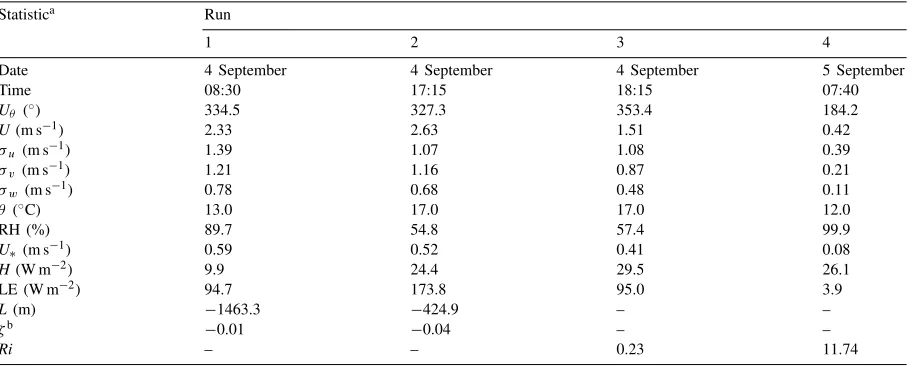
Table 3
Atmospheric conditions measured at 30 m above ground (10 m above the forest) during the spray runs
Statistica Run
1 2 3 4
Date 4 September 4 September 4 September 5 September
Time 08:30 17:15 18:15 07:40
Uθ (◦) 334.5 327.3 353.4 184.2
aThese are 30 min average statistics rotated into the mean wind stream. Wind direction is represented byUθand was determined before the rotations. Mean wind speed isU. Standard deviations of the steamwise, cross-stream and vertical wind components areσu,σv, andσw. θis the virtual air temperature. RH is the relative humidity. The friction velocity,u∗, was calculated as [u∗=(u′w′)0.5] whereu′w′was the
uwcovariance. The sensible heat flux,H, was calculated from [H=ρcp(θ′w′)] whereθ′w′ was theθwcovariance,ρ, the air density was
1.205 kg m−3andcp, the specific heat of air was 1000 J kg−1. The latent heat flux, LE, was calculated from [LE=ρwLv(w′q′)] whereρ
wwas
the density of water, andLv, the latent heat of vaporization, was 2.45×10⁶J kg−1.Lis the Monin–Obukov length [L= −(ρcpθu∗3)/(kgH)]
wherekis the von Karman constant (0.4) andgis the acceleration due to gravity.ζ is the stability parameter [ζ=(z−d)/L] wherezin this case is 30 m anddis the zero plane displacement, 14 m.Riis the Richardson number for the roughness sublayer above the forest.Ri was calculated as [Ri=(g/θ)(1θ/1z)/(1U/1z)2] where the gradients1θand1Uare measured between heights of 30 and 22 m,1z=8 m. bζ was used to quantify stability when the overall boundary layer was convective andRiwas unreliable due to advection over the forest edge.Riwas used during the transition periods whenLandζ are undefined in the surface layer.
4.2. The suspension and movement of droplets in air
The suspension of sparya droplets in the air is de-termined by the size (aerodynamic diameter) of the droplet and the turbulence intensity of the air flow (Bache and Johnstone, 1992). Large dropssettle out of the air rather quickly; that is, in less than 30 s from standard spary heights. Small drops stay suspended in the air and do not settle out. Drops are defined as large when their settling velocity,vs> 0.3u∗(u∗is the
friction velocity of the air, a measure of turbulence which helps to keep the droplet suspended). Drops are defined as small when vs<0.3u∗. Since u∗ above a
forest increases with higher wind speeds and rougher canopies (Miller et al., 1995), a drop defined as large in a 1 m s−1wind may not be a large drop in a 5 m s−1 wind. Also, a drop might settle from the air over a short canopy but remain suspended over a forest due to the difference in u∗ over each canopy type.
Air-borne drops become rapidly smaller by evaporation,
decreasingvsand increasing the chances of remaining
airborne. When suspended in the air, the droplets evap-orate at the same rate as water, with corresponding re-duction in size, until the water fraction is gone and the non-volatile ingredients are conserved in the drop. All of the models listed earlier calculate reduction of drop size by evaporation using this conserved ‘hard-core’ approach. The suspended material is not easily de-tected with passive samplers because it will not impact a surface easily or settle out of the air stream.
Fig. 6. Peak plume density decay rates for nine independent spray swaths.
and it is easier to obtain complete coverage of the target area under these conditions. Our measurements imply that the smaller droplets remain suspended dur-ing these transition and calm periods and the plumes spread slowly until the atmospheric conditions change and increase the dispersion rates.
Low winds together with unstable conditions caused the plumes to spread vertically very rapidly with por-tions of the plume breaking off and moving upward in the convective atmosphere. Moderate winds with unstable conditions moved the plume away from the spray area at the mean wind speed and spread the plume equally rapidly in both the horizontal and verti-cal directions. Fig. 6 graphiverti-cally demonstrates the ef-fect of stability on plume dissipation rate. The swaths are grouped by stability into two families of curves where the plume densities decrease rapidly in unstable conditions and slowly in stable conditions.
Only one circumstance showed the possibility of higher capture of the small droplets at the site. When the plume moved over the forest, the vertical location
4.3. Implication for control of long range dispersion of pesticides
These measurements imply that even well managed spray operations contribute to the general air pollution load of pesticides. Thus, the worldwide occurrences of traces of pesticides may not just be due to volatiliza-tion, accidents, careless applications or poor training of applicators. Although this study does not quantify a connection between normal spray operations and the widespread dispersal of pesticides, or their degrada-tion products, in the environment, it does indicate that one exists. If so, this problem cannot be completely controlled with the current technology and manage-ment procedures.
5. Conclusions
Lidar scans indicate regions of backscatter per-sisting in the atmosphere and drifting off after the larger drops should have settled out. We infer that this backscatter represents droplets less than 80–100m
diameter. These plumes of small droplets remain sus-pended in the air and drift off after every aerial spray application. Some small droplets dispersed into the atmospheric boundary layer in all the cases studied. Thus, even well managed spray applications can con-tribute to the general air pollutant load of pesticides. Plume movement and the rate of near-field plume dilution depends primarily on the stability of the at-mosphere, which implies that high concentrations in the air in adjacent areas can be partially controlled by correct timing of the spray operations.
Acknowledgements
The authors especially thank Dr. William Eichinger, University of Iowa, for the use of his lidar software. This research was supported in part by the US Army Research Office grants DAAG55-97-1-0048 and DAAH-4-95-0319; in part by the USDA Forest Ser-vice, Northeast Forest Experiment Station (NEFES) and the National Forest Health through Center Coop agreement 23-250 and in part by the US EPA Grant CR823627-010-1. USDA Animal and Plant Health Inspection Service provided the aircraft and pilot and the USDA FS NEFES provided the spray material.
This was a joint project of the Environmental Research Institute at the University of Connecticut and the Storrs Agricultural Experiment Station. This is paper 1816 of the Storrs Agricultural Experiment Station.
References
Aylor, D.E., 1998. Documentation of a two-dimensional Lagrangian simulation mode of pesticide spray drift in an orchard canopy. Tech. Rpt. The Connecticut Agricultural Experiment Station, New Haven CT, 63p. ****
Bache, D.H., Johnstone, D.R., 1992. Microclimate and Spray Dispersion, Ellis Horwood, Chichester, Uk, 139p.
Baldocchi, D.D., Meyers, T.P., 1988. Turbulence structure in a deciduous forest. Boundary Layer Meteorol. 43, 345–364. Carson, R., 1962. Silent Spring, Houghton Mifflin, Boston, MA,
368p.
Fox, R.D., Derksen, R.C., Brazee, R.D., 1998. Air-blast/air-assisted application equipment and drift. Proc. National Spray Drift Conference, Univ. Maine Extension Service.
Hewitt, A.J., Valcore, D.L., Esterly, D., Teske, M.E., 1997. ‘What if’ drift mitigation scenarios with the agdrift model. American Society of Agriculture Engineers meeting presentation paper # 971073, 16p.
Holst, R.W., Ellwnager, T.C., 1984. Pub. EPA-540/9-84-002. US Environmental Protection Agency, Washington DC.
Kurtz, D.A. (Ed.), 1962. Long Range Transport of Pesticides, Lewis Publishers, Chelsea, MI.
Majewski, M.S., Capel, P.D., 1995. Pesticides in the atmosphere. In: Gilliom, R.J. (Ed.), Series Pesticides in the Hydrologic System, Vol. 1, Ann Arbor Science, Ann Arbor, MI. Miller, D.R., Reardon, R.C., McManus, M.L., 1995. An
Atmospheric Primer for Aerial Spraying of Forests. USDA Forest Service, National Center for Forest Health Management FHM-NC-07–95, 19p.
Miller, D.R., Yendol, W.E., Ducharme, K.M., Maczuga, S., Reardon, R.C., McManus, M.A., 1996. Drift of Aerial Applied Diflubenzuron Over an Oak Forest. Agric. & For. Meteorol. 77. Picot, J.J.C., Kristmanson, D.D., 1997. Forestry Pesticide Aerial
Spraying, Kluwer Academic Publishers, Dordrecht, 213p. Somasundurama, L., Coats, J. (Eds.), 1991. Pesticide
Transformation Products, Fate and significance in the Environment, American Chemical Society, Washington DC. Spray Drift Task Force, 1997. Summaries of Application Studies.
Steward Agricultural Research Services, Macon, Missouri. Stoughton, T.E., Miller, D.R., Yang, Y., Ducharme, K.M., 1997.
A comparison of spray drift predictions to lidar data. Agric. For. Meteorol. 88, 15–26.
Teske, M.E., Bowers, J.F., Rafferty, J.E., Barry, J.M., 1992. FSCBG: an aerial spray dispersion model for predicting the fate of released material behind aircraft. Enviro. Toxic. Chem. 12 (3), 453–464.
Walklate, P.J., 1992. A simulation study of pesticide drift from an air-assisted orchard sprayer. J. Agri. Eng. Res. 51, 263–283. Wang, Y., Miller, D.R., Anderson, D.E., McManus, M.L., 1995.