Practical implementation of the fractional flow
approach to multi-phase flow simulation
Philip Binning
a ,* & Michael A. Celia
b aDepartment of Civil, Surveying and Environmental Engineering, The University of Newcastle, Callaghan, N.S.W. 2308, Australia b
Department of Civil Engineering and Operations Research, Princeton University, Princeton, NJ 08544, USA
(Received 13 August 1997; revised 24 June 1998; accepted 30 June 1998)
Fractional flow formulations of the multi-phase flow equations exhibit several attractive attributes for numerical simulations. The governing equations are a saturation equation having an advection diffusion form, for which characteristic methods are suited, and a global pressure equation whose form is elliptic. The fractional flow approach to the governing equations is compared with other approaches and the implication of equation form for numerical methods discussed. The fractional flow equations are solved with a modified method of characteristics for the saturation equation and a finite element method for the pressure equation. An iterative algorithm for determination of the general boundary conditions is implemented. Comparisons are made with a numerical method based on the two-pressure formulation of the governing equations. While the fractional flow approach is attractive for model problems, the performance of numerical methods based on these equations is relatively poor when the method is applied to general boundary conditions. We expect similar difficulties with the fractional flow approach for more general problems involving heterogenous material properties and multiple spatial dimensions.q1999 Elsevier Science Ltd. All rights reserved.
Keywords: multi-phase fluid flow, numerical methods, fractional flow, MMOC.
1 INTRODUCTION
Numerical simulation of multi-phase flow in complex porous media remains one of the outstanding difficulties in the field of computational hydrology. The reasons for this difficulty include the highly nonlinear nature of the coupled partial differential equations that govern the system, and the lack of reliable constitutive data for these problems. This difficulty has led many researchers to explore alternative forms of the governing equations, and to seek specialized numerical algorithms that can improve the computational performance of a simulator.
Historically, there have been two main approaches to modeling multi-phase flow, arising in the disciplines of hydrology and petroleum engineering. The first is based on individual balance equations for each of the fluids, while the second involves manipulation and combination of those balance equations into modified forms, with
concomitant introduction of ancillary functions such as the fractional flow function. The latter approach derives almost exclusively from the petroleum literature. In 1973, Morel-Seytoux1wrote a classic paper in which he drew together much of the previous research and explored unifying themes between the disciplines. He showed that the flow of air and water in unsaturated soils can be viewed as a multi-phase system, and showed how the experience of petroleum engineering could aid in understanding of multi-phase flow problems in hydrology. Since then many developments have occurred, particularly in the area of numerical methods for the solution of the multi-phase flow equations.
Numerical methods are very sensitive to the choice of form of the governing equation. Morel-Seytoux1 showed that there are several ways to write the governing equations of fluid flow, and that each method offered its own insights into the solution. More recently, Ewing2has also examined recent developments in the choice of equation form for multi-phase flow. In the light of the new and continuing developments in numerical methods for the solution of the
Printed in Great Britain. All rights reserved 0309-1708/99/$ - see front matter
PII: S 0 3 0 9 - 1 7 0 8 ( 9 8 ) 0 0 0 2 2 - 0
multi-phase flow equations, it is worthwhile revisiting the question of the form of the governing equations and explor-ing the implications of this equation form for a numerical method based on it.
Two approaches to writing the governing equations will be examined here: the two-pressure approach; and the frac-tional flow approach. The two-pressure approach to the governing equations has been widely used in the hydrologic literature. In this approach, the governing equations are written in terms of the pressures in each of the two phases through a straightforward substitution of Darcy’s equation into the mass balance equations for each phase. This approach has been adopted by a number of authors includ-ing: Pinder and Abriola3who employed a finite difference approximation of the governing equations to describe non-aqueous phase liquid flow in the saturated zone; Sleep and Sykes4, and Kaluarachchi and Parker5, who used a finite-element solver with a Newton–Raphson scheme to linearize the equations; Celia and Binning6–8who employed a finite element discretization with fully implicit time stepping and Picard iteration to solve the air and water flow equations; and Schrefler and Xiaoyong9, who solved the consolidation problem in the unsaturated zone with a finite element discretization of the governing equations.
The fractional flow approach originated in the petroleum engineering literature, and employs the saturation of one of the phases and a pressure as the independent variables. The fractional flow approach treats the multi-phase flow problem as a total fluid flow of a single mixed fluid, and then describes the individual phases as fractions of the total flow. This approach leads to two equations: the pressure equation; and the saturation equation. The pressure equation is an elliptic equation that is solved for the pressures and the total flux. The saturation equation is written in advection– diffusion form with a hyperbolic characteristic that describes the speed of an infiltrating front. The advective term is nonlinear and usually leads to shock formations. Its general behavior may be exploited to design a Lagrangian numerical algorithm that allows for relatively large time steps by projecting the solution forward along the characteristics.
In the absence of capillarity and gravity, the saturation equation may be solved analytically; this approach dates to Buckley and Leverett10. Interest in the saturation equation and its analytic solution continues today. For example, Sander et al.11 have found an analytic solution for a restricted class of functional forms. Numerical solutions have been considered more recently. Morel-Seytoux and Billica12,13, and Wangen14used finite difference methods, and Chen et al.15 employed finite elements and mixed methods to solve the fractional flow equation for one-dimensional systems with incompressible fluids, while a general characteristic-based approach was presented by Douglas16 and Espedal and Ewing17. The computational work of Dahle et al.18,19, Celia and Binning20, and Langlo and Espedal21demonstrated the computational benefits of the characteristic-based method, with the paper by Langlo and Espedal22 presenting simulation results in two
dimensions with variability in the intrinsic permeability of the medium. Hansen et al.23 considered systematic treat-ment of the gravity terms in the fractional flow formulation. The problem of boundary condition implementation has also been considered recently by Chen et al.24.
The pressure equation has been solved by a variety of methods. In one dimension, for incompressible flow the total velocity is a constant in space that depends only on the time varying boundary conditions, and so the pressure equation may be solved analytically1. In higher dimensions, numerical methods must be employed. Ewing25 reviews numerical techniques for solution of the pressure equation and demonstrates the importance of accurate determination of velocities. Variations in material properties, particularly the permeability, can cause sharp changes in pressures. Large errors can result if these pressures are differentiated
to obtain the necessary velocities. Ewing and
Heinemann26,27developed a mixed method for solution of the pressure equation, with the aim of accurate determi-nation of velocities. They showed that mixed methods were far superior to conventional approaches when applied to standard five-spot problems. Mixed methods are the state-of-the-art at the current time.
Other approaches to the numerical solution of the frac-tional flow equations include the work of Guarnaccia and Pinder,28 who employed the fractional flow formulation with the sequential solution method of Spillette et al.29to decouple the equations and a collocation method to dis-cretize the equations to solve the problem of NAPL migration in the water and gas phases.
While the fractional flow and two-pressure approaches have been studied by various researchers, other methods have also been developed to solve multi-phase flow equations. One of the more important variants on these methods is the pressure–saturation approach. Since the saturation is a function of the capillary pressure or differ-ence between phase pressures, it is possible to reformulate the governing equations in terms of a saturation and one of the phase pressures. The second phase pressure can then be removed from the equations by expressing it in terms of the saturation and the pressure in the other phase. The attraction of this approach is that it is very well suited to problems where there may be phase disappearance. If the saturation in one of the phases is zero, the pressure in that phase is poorly defined. A standard two-pressure formulation will not be able to handle this problem. The pressure saturation
approach has been employed by Faust,30 Kueper and
Since the governing equations for multi-phase flow are highly nonlinear, numerical techniques must in general be employed for their solution. There are many choices of numerical method, with temporal discretization being a topic of great interest in the literature. In hydrologic appli-cations the predominant approach has been to employ fully implicit schemes. Haverkamp et al.37 compared temporal discretizations of Richards’ equation, and showed that because of the stability restrictions on explicit solvers, implicit solvers provide solutions five to ten times faster than explicit solvers. The better performance of the implicit solvers occurs, despite the need for iterations to deal with the nonlinearities. Multi-phase flow simulators in hydrology have similar behavior to that observed by Haverkamp, and so fully-implicit time stepping is the dominant approach in hydrology and has been adopted by many authors36,38.
The petroleum engineering literature contrasts with the hydrology literature with the predominant approach being explicit or semi-implicit. The most common approach employed38 is the IMPES scheme (implicit pressure, explicit saturation). This scheme has been favored because it decouples the pressure and saturation equations, thus reducing the computational effort required for their solution. The IMPES scheme has been used by Sleep and Sykes39 who used it to simulate the behavior of an air–water system. Sleep and Sykes compared the efficiency of an IMPES scheme with a fully implicit scheme. They showed that the IMPES was more restricted in time step size than the implicit scheme. The difference in time step size made up for any speed the IMPES gained by decoupling the equations. However, the IMPES scheme requires less memory, which may be a consideration for larger problems. A new development in hydrology is the use of an adaptive implicit scheme, which was first employed in the petroleum literature. A fully implicit formulation is used in regions of sharp changes of independent variables and the explicit scheme used elsewhere. An example is the work of Reeves and Abriola.40
In this paper, the equations that describe two-phase fluid flow will be reviewed. The equations will be presented in a two-pressure, or standard mass balance, form that is com-monly used by hydrologists, as well as a modified form that we will refer to as the fractional flow or global pressure– saturation form that has been developed by petroleum engineers. Computations will be used to demonstrate the differences in performance between numerical approxima-tions of the different equation forms, and the implicaapproxima-tions for the future multi-phase modeling efforts discussed. The paper will not discuss the various choices of temporal dis-cretization, as these are examined in other works. A fully implicit time discretization will be adopted for all numerical schemes, and the focus of the paper will be on the form of the governing equation and the implications of that form on the performance of the numerical method.
The paper will also consider questions related to practical implementation of the fractional flow approach to multi-phase flow simulation. In particular, we will revisit the
question of general boundary conditions, consider the impli-cations of general material heterogeneities, speculate on the potential difficulties with multiple infiltration and drainage fronts, and consider some general questions related to fluid compressibility and gravity terms.
2 GOVERNING EQUATIONS
In this presentation, we consider balance and constitutive equations applicable to each fluid phase; we will not con-sider modeling of individual components or processes of interphase transfer. For each fluid phasea, the mass balance equation may be written as
](raJSa)
]t þ=·(raqa)¼0 (1)
whererais the density of fluida,Jis porosity, Sais fluid
saturation, and qais the volumetric flux vector for phasea.
For a two-fluid-phase system, eqn (1) is written for each fluid phase, and is augmented by constitutive relationships that relate saturations to capillary pressure (eqn (2)), specify a closure condition on saturations (eqn (3)), and relate volumetric fluxes to pressure gradients via a multi-phase version of the Darcy equation (eqn (4)) which includes relative permeabilities (eqn (5)),
Sa¼Sa(pc)¼Sa(pnw¹pw) (2)
the individual phase pressures with w and nw denoting the wetting and non-wetting phases respectively, k is the intrin-sic permeability tensor,mais the viscosity in phasea, g is
the gravitational vector (the vertical coordinate is oriented positive down), and krais the relative permeability to phase
a which is a nonlinear function of saturation.
If fluid or matrix compressibility is considered, then appropriate compressibility coefficients also need to be defined. For the purposes of this paper all fluids, as well as the solid matrix, will be considered to be incompressible. Given this set of equations, boundary and initial condi-tions must be supplied to complete the mathematical description. These are usually given as known pressures, saturations or fluxes in each of the fluid phases. Many dif-ferent combinations of these boundary conditions occur in practical problems. An important criteria for acceptance of a numerical method is that it must be able to solve the govern-ing equations for the wide variety of possible boundary conditions.
alternate forms with various choices of primary dependent variables. The choice of equation form and primary solution variables have considerable implications for the numerical method used to solve the equations. Two possible formula-tions will be considered here and the benefits of each discussed. In the two-pressure formulation, the pressures in each phase are chosen as independent variables and the governing equations are parabolic in nature. The other formulation employed is the fractional flow approach where a saturation and a ‘global pressure’ are chosen as independent variables. In this case, the governing equation for saturation is parabolic (hyperbolic in the case of zero capillarity) and the equation for pressure elliptic.
2.1 Two-pressure approach
The conventional approach to solving the governing equations, eqns (1)–(5) in hydrology involves a straight-forward substitution of the Darcy equation (eqn (4)) into the mass balance equation (eqn (1)) to eliminate the fluxes from the equations. The primary unknowns are chosen to be the two phase pressures, pwand pn w. The saturation in the non-wetting phase is eliminated using eqn (3).
J]Sw
The equations are coupled and nonlinear, and are closed by specification of the pressure–saturation relation (eqn (2)) and relative permeability relation (eqn (5)).
2.2 Fractional flow approach
The fractional flow approach is again based on a set of two nonlinear equations, each of which has its origin in eqns (1)–(5), but with a different choice of dependent variables. Definition of these variables requires extensive manipula-tion and rearrangement of the two-phase equamanipula-tions. For simplicity of presentation, consider the case of constant fluid densities and constant porosity. Then the individual phase mass-balance equations (eqn (1)) sum to form
=·(qwþqnw)¼=·qT¼0 (8)
where qT, called the total flux, is the sum of the
phase-volumetric fluxes. In one dimension this equation has the particularly simple solution that the total flux is a constant in space determined by the boundary conditions. A new independent variable is now introduced, called the global pressure, with the aim of expressing the total flux solely in terms of the gradient of the global pressure and not in terms of the individual phase pressures. Following Chavent and Jaffre´,41a global pressure is defined by
P¼1
Given these definitions, the total velocity may be related to the total pressure.41 This expression for the total velocity may then be substituted into eqn (8) to obtain the nonlinear elliptic partial differential equation that governs the evolution of the total pressure P,
=·L·=P¹=·(LG)¼0 (11)
is the total mobility coefficient, and
G(Sw);(fwrwþ(1¹fw)rnw)g
is a nonlinear function of saturation that accounts for gravitational effects. Eqn (11) forms the first of the two governing equations in the fractional flow approach.
The second equation used in the fractional-flow equation set is derived from manipulation of eqn (1) witha¼w, such
that the primary dependent variable is wetting-phase satura-tion Sw. Because eqn (1) contains an individual phase flux that is dependent on an individual phase pressure, an equation is found relating the individual phase flux, qwto the total flux
In eqn (12),Fwis the fractional flow function incorporating both gravity and capillarity. In one dimension, substitution of eqn (12) into eqn (1) witha¼w, and assuming
incompres-sible flow, results in the following saturation equation.1,41
J]Sw
The coefficient D(Sw) is the capillary diffusion term, while Fwis the fractional flow, containing fwas well as the gravity drive, and is defined so that qw¼Fw(Sw,P) in the absence of capillary forces. The definition Fwdegenerates into qTfwin the absence of gravity. Note that the definition of Fwin eqn (14) differs slightly from that of Chavent and Jaffre´41and Morel Seytoux,1 whose definition is divided by the total flux qT. The equation form presented here follows the
qTin Fw, in order that it remained well defined in the case of zero total flux.
When eqns (11) and (13) are supplemented with appro-priate boundary conditions, they may be solved for the unknowns P and Sw. Implementation of boundary con-ditions is discussed below. The equations are coupled through the dependence of the nonlinear coefficients L and G in the pressure equation on the saturation Sw and through the dependence of the total velocity qTappearing
in the saturation equation on the global pressure P. Note that the definition of global pressure means that the pressure and saturation equations are only loosely coupled. Other defini-tions of pressure and saturation will increase the coupling between the equations. The other advantage of the choice of global pressure and saturation as independent variables is that these variables are smoother than the individual phase pressures, and so the performance of numerical methods based on these equations should in principle be better than solvers employing phase pressures as the independent variables.2
In an oil–water system, with typical relative permeability functions given by18,42
krw¼S
3
w (16)
krnw¼(1¹Sw)
3
(17)
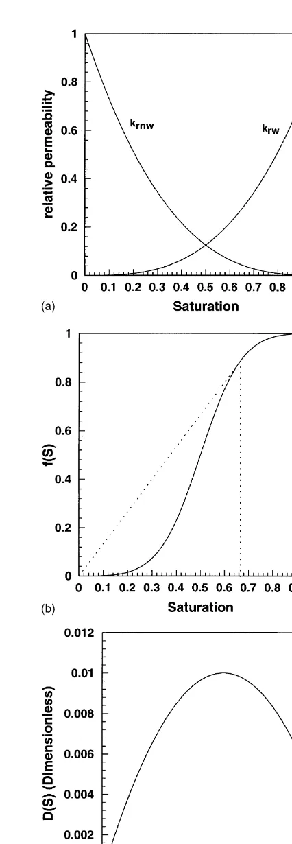
the fractional flow function has characteristic S-shape, in the absence of gravity and assuming equal fluid viscosities. Fig. 1 shows both the relative permeability functions and the fractional flow function f. This S-shaped fractional flow function leads to solutions that combine a shock front with a rarefaction wave when gravity is absent; this is the classical Buckley–Leverett solution. When capillary diffu-sion is considered, the front exhibits some spreading, but this is often relatively minor. Fig. 2 shows the Buckley– Leverett solution, together with the full solution of the saturation equation with permeabilities given by eqns (16) and (17) and D(Sw)¼0.04«Sw(1¹Sw) with«¼0.01 (See Dahle18 for details of these functional forms). In either case, the frontal speed may be estimated from the classic theory of hyperbolic equations.
For an air–water system the fractional flow and capillary diffusion functions are quite different from the oil–water case, because of the much higher viscosity difference between fluids. For air and watermw ¼0.001 N s m
¹2and
ma¼ 1.833 10
¹5N s m¹2 at 208C, leading to a mobility
ratio of 54.6, as opposed to the oil–water system above, which was modeled with a mobility ratio of 1. As pointed out by Morel Seytoux,1this viscosity contrast causes both curves to shift significantly toward the higher water saturations, greatly diminishing the rarefaction wave and expanding the shock range. As an example, the relative permeability functional forms determined experimentally by Touma and Vauclin43 are used to derive the fractional flow and capillary diffusion functions. The appropriate
functional forms, determined experimentally by
Touma and Vauclin, are as follows: the capillary
Fig. 1. Functional forms of Young42and Dahle et al.18for an oil– water system. (a) Relative permeability curves. (b) Fractional flow function. The slope of the Welge49tangent line drawn gives the speed of shock fronts formed in the solution. (c) Approximate
pressure–saturation relationship, obtained by fitting a van Genuchten44form to the data, is
Sw¼
androwis the density of water at standard temperature and
pressure. For the hydraulic conductivities, Touma and Vauclin fitted a polynomial to experimental observations with the results: the saturated conductivity of water Kw s ¼ 15.40 cm h
¹1;
Aa ¼ 3.86 3 10
¹5; and the saturated conductivity of air
is Ka s¼2800 cm h
¹1. The air and water functional forms
are shown in Fig. 3. The figure is plotted using the normal-ized water saturation S¼ Sw¹Swr
Sws¹Swr. The water relative
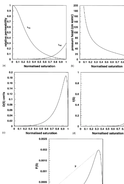
perme-ability does not reach kr w ¼ 1 because the maximum saturation Sw s is less than 1 during infiltration. The figure also shows the fractional flow function and the capillary diffusion function.
3 NUMERICAL METHODS
Three numerical methods are presented. The first solves eqns (6) and (7) and is called a two-pressure solution. The
second and third solve the fractional flow equations (eqns (11) and (13)) using a finite difference and characteristics formulation. All numerical results are
presented here for one-dimensional problems. The
two-pressure solution has been generalized to higher dimensions.45 The numerical solutions of the fractional flow equations (eqns (11) and (13)) have not been extended to higher dimensions using the methodology presented here, although several other authors have presented
solutions to the saturation equation (eqn (13)) in
two-dimensions.18,22,46,47
3.1 Solution of two-pressure equations
The two-pressure equation formulation was employed by Celia and Binning6 in their numerical simulation of two-phase air and water flow in the unsaturated zone. Their method is based on a finite element discretization in space, a backward Euler approximation in time, and a so-called modified Picard linearization. With superscripts n and
m denoting time level and iteration level, respectively, the
time-discretized equation takes the following form (see Celia and Binning for details):
J:dSw
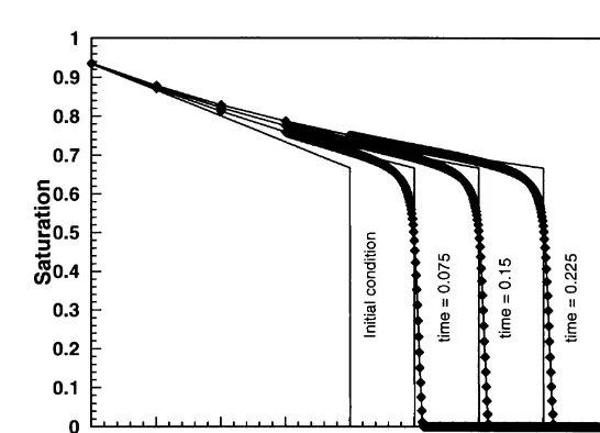
Fig. 2. Solution of the saturation eqn 13) using the oil–water functional relationships shown in Fig. 1. The MMOC solution of the full saturation equation is shown as a line with nodal positions marked. The Buckley–Leverett solution is shown as a solid line for comparison.
Fig. 3. Functional forms of Touma and Vauclin43for air and water in a coarse sand. (a) Relative permeabilities. (b) Pressure saturation curve. (c) Capillary diffusion function. (d) Fractional flow function f. (e) Fractional flow function F for the case qT¼0. The dashed line is
¹J:dSw
These equations are linearized with unknowns dpnwþ1,m anddpnaþ1,m. The right hand side R
nþ1,m
a is a function of
the known pressures at the new time level and old iteration (nþ1,m) and old time (n) levels. At each iteration step the equations are solved and the dpnaþ1,m used to update the pressures. Iteration proceeds until the residual Rnaþ1,m given by the right hand side of each equation reaches a user specified error tolerance. The residual can be seen to be a measure of the degree to which the numerical solution satisfies the governing equation.
To complete the discretization, a spatial approximation is required. A lumped Galerkin finite element discretization is chosen using piecewise linear basis functions. Lumping of the mass matrix is useful in controlling oscillations that arise through the finite-element discretization of the time derivative. The numerical equations are solved simul-taneously for the air and water pressures, with the air and water equations at each node being written alternately in the matrix formation. This leads to a five-banded block symmetric matrix.
3.2 Numerical solution of the fractional flow equations
The fractional flow approach comprises two equations—the pressure equation (eqn (11)) and the saturation equation (eqn (13)). These equations present a greater numerical challenge than those of the two-pressure approach. The two-pressure approach involves two equations with a simi-lar mathematical character, and so the same numerical method can be used for both equations leading to a simple numerical technique. In contrast, the fractional flow approach involves two equations with completely different characters, and so separate numerical techniques must be devised for each equation.
3.2.1 Saturation equation
One of the main attractions of the fractional flow approach is the form of the nonlinear advection term in eqn (13). The family of characteristics associated with the hyperbolic part of these equations provide the physically-correct speed for an infiltrating front. Numerical methods may be developed to take advantages of this information, thereby leading to potentially improved numerical performance. Two methods of solution of the saturation equation are presented here. The
first is an Eulerian approach due to Morel-Seytoux and Billica,12,13 who employed a simple finite difference scheme. The second is an Eulerian–Lagrangian approach that solves the saturation equation using a modified method of characteristics (MMOC).
3.2.2 Finite difference solution of the saturation equation
The finite difference scheme developed by Morel-Seytoux and Billica employs a centered-in-space discretization and a Euler backward time stepping, with a Picard iteration scheme for the nonlinear coefficients. For evenly spaced nodes and a constant (in space) total velocity, the scheme can be written
where j is an index over space, n denotes the time level, and
m the iteration level.
3.2.3 MMOC solution of the saturation equation
While the finite difference approximation (eqn (20)) has certain benefits, especially for one-dimensional problems, it ignores the fact that the hyperbolic part of the saturation equation may be solved by numerical methods that take advantage of the secondary (hyperbolic) characteristics of eqn (13). The total flux is constant in one dimension and smooth in higher dimensions, and so an infiltrating front of the wetting fluid will move at a fairly uniform velocity with a fairly constant shape.
The saturation equation (eqn (13)) can be solved by a characteristic-based approximation. One such method, based on the MMOC with localized grid refinement, was outlined and implemented by Celia and Binning for the case of known qTand simple boundary conditions. Other similar
approaches include the recent Eulerian–Lagrangian loca-lized adjoint method (ELLAM) approach of Dahle et al.,48 as well as earlier work of Dahle,18Espedal and Ewing,17and others cited earlier in this paper. The procedure used herein is an extension of the MMOC approach outlined in Celia and Binning.20 The key enhancements to the original algorithm of Espedal and Ewing17include the changed defi-nition of Fwso that it remains well defined in the case of zero total flux, the definition of operator splitting for growing infiltration fronts, and the development of an algorithm to handle general boundary conditions.
(eqn (13)), which we will rewrite:
is the material derivative of saturation. The hyperbolic part of the equation DSw
Dt ¼0 is nonlinear and produces solutions
with shocks, although these shocks (or fronts) move with well-defined speed. This frontal speed is calculated using the convex envelope of the fractional flow function through the following algorithm. The saturation equation is split into two equations
where the new functions ¯F9and b are defined in order that the equation DSw
Dt ¼0 gives the physical frontal speed. Eqn (23) can be termed a ‘characteristic equation’ and eqn (24) a ‘diffusion correction equation’. The correct definitions for ¯F(Sw) and b(Sw) are found by examining the Buckley– Leverett solution to the equation. This leads to the following definition:
and b(Sw) is defined in the appropriate manner. Note that the above splitting is based on the assumption that Fw(Sw) is concave for Sw$ S
t w.
The simulations presented in this paper are all one-dimensional. Splitting in the higher-dimensional case including gravity has been considered by Hansen47 and Hansen et al.23 The function ¯F(Sw) for oil and water, as used by Dahle,18 is shown in Fig. 1b, as the concave envelope of the fractional flow function.
While the shock is never fully developed for problems with non-zero capillary diffusion, the algorithm is designed to assume that the infiltrating front is fully developed, so that the Buckley–Leverett saturation is used for Stw. The Buckley–Leverett saturation is found using the tangent law of Welge49which solves the equation
F(Sw)
Sw
¹dFw
dSw
¼0 (26)
for the Buckley–Leverett saturation SBL. If the maximum
saturation in the domain is less than the Buckley–Leverett saturation then Stw is reduced to this lower value.
The operator splitting discussed above is for the case of the wetting fluid infiltrating into non-wetting fluid. Under drainage, and combined drainage–infiltration events, the definition needs to be modified. The discussion of these modifications is beyond the scope of this work. Questions also arise in heterogeneous materials where the character-istics cross the boundaries between two materials having different fractional flow function definitions. It is not clear how this would be handled with the current method. While the work of Langlo and Espedal22 addresses the issue of heterogeneity, it avoids this problem by using hetero-geneous materials where only the absolute permeability varies, with the nonlinear functional forms remaining the same.
Numerically, eqns (23) and (24) are solved separately
18,50. The characteristic eqn (23) is solved using a
character-istic algorithm, and the diffusion correction eqn (24) is solved using a spatially optimal Petrov–Galerkin finite element method.
The first step in the numerical algorithm is the numerical determination of the operator splitting. This is done by find-ing Stw and S
b
w. Eqn (26) is solved using the method of bisection and the result compared to the maximum satura-tion in the domain to define Stwas above. S
b
wis defined to be the minimum saturation in the domain.
Localized grid refinement is very attractive with a Lagrangian approach to the governing equations. The saturation equation can be solved analytically for frontal speed, and the speed used a priori to refine the grid at the projected location of the infiltrating front at the new time step. The frontal location is defined by examining the gradient of saturation. In regions where the grid has been refined but the gradient of the solution is no longer large, the mesh refinement is removed.
The characteristic equation (eqn (23)) is solved by back-tracking along characteristics from the new time level to find the characteristic solution S¯n17. Because the velocity of the front is a function of the saturation, an iterative scheme must be employed to find the correct solution. Note that a major source of error in the numerical solution is through the interpolation of the saturation to grid locations inbetween nodes.
The material derivative in the diffusion correction equation is then approximated using the characteristic solution and the diffusion correction equation is written as
JS
domain into E elements Qe ¼ [ze,zeþ1]. Piecewise linear
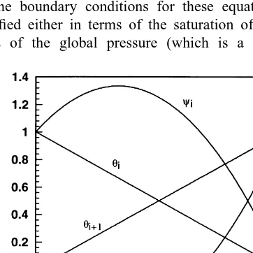
basis functions, vi, and spatially ‘optimal’ test functions, wi are used, with sufficient upstream weighting added to provide enough artificial diffusion at the solution front so that non-unique solutions do not form.50The test functions are weighted ‘upstream’ in relation to the b(Snwþ1,m)term, which is an advection term in the opposite direction to the flow. Fig. 4 shows a fully upstream weighted test function for a front that is moving from left to right (since b is an advection term that sharpens the front it is in the opposite direction to the frontal movement). Within the Petrov– Galerkin procedure, the temporal derivatives are lumped using the L1 scheme of Milly,51 and the grouped term b(S)S is expanded using the finite element representation. The resultant algebraic system is tridiagonal in structure, and is solved using the Thomas algorithm. See Binning45 for details.
3.3 Solution of pressure equation
Compared to the saturation equation the pressure equation is very well behaved. The pressure equation is a highly non-linear elliptic equation. The pressure, however, is relatively smooth and the numerical approximation is straightforward. Since all simulations presented here are for a homogeneous medium, a simple Galerkin finite element method with piecewise linear basis functions is used instead of the mixed methods of Ewing and Heinemann.27
3.4 Treatment of boundary conditions
If the fractional flow approach is applied to general multi-dimensional, incompressible fluid flow problems, the appropriate equations are the pressure equation (eqn (11)), and the saturation equation (eqn (13)). This set of equations is solved for the water saturation, Sw, and the global pressure,
P. The boundary conditions for these equations can be
specified either in terms of the saturation of water or in terms of the global pressure (which is a non-physical
variable). Boundary conditions may also be specified in terms of the total flux qT (or gradients of P). The
total-flux-type boundary condition is often used in simulations of petroleum reservoirs. In petroleum reservoirs the total flux can conveniently be specified as zero, as the domain of simulation is often enclosed by no-flow boundaries (for example in a five-spot problem).
In hydrology, complex boundary conditions involving combinations of individual fluid fluxes or pressures often must be specified. These types of boundary conditions at the land surface are difficult to implement using the fractional flow form of the equations, because of the non-physical nature of the global pressure. For example, for infiltration problems, the boundary conditions at the land surface are typically specified as a given air pressure and a water flux. From these two values, neither P nor Swcan be calculated.
In one-dimensional problems it is possible to derive analytically an expression for total flux1. Because we wish to develop algorithms that are applicable to higher-dimensional problems, where analytical expressions are not available, we will not employ the analytical expressions in the one-dimensional problem. Rather, a more general technique will be developed.
An iterative technique is required for implementation of general boundary conditions. Consider the case where the flux of wetting phase qw and pressure of the non-wetting phase pnware known at the top boundary and the saturation and global pressure are specified at the lower boundary. In this case the saturation and global pressure within the domain, boundary conditions at the top end of the column and the total velocity are unknown. An iterative solution for
P, Swand qTin the interior and P and Swat the boundary is developed. The procedure can be described as follows:
1. Begin the solution by estimating the total flux by using the known wetting phase boundary flux qT ¼ qw.
2. Next estimate Stop, the saturation at the top boundary
by dividing the given value of qw by the saturated hydraulic conductivity. Use this ratio as a guess for
krw, and determine the value of Stop implied by
that value of krw. Mathematically, solve
qw
krowg=mw¹krw(Stop)¼0 for the saturation Stop at
the top boundary.
3. Given Stop at the boundary solve the saturation
eqn (13) using MMOC.
4. Given the solution Sw, calculate the capillary pressure at the top boundary, then with the given pa at the boundary, calculate pw. Now with pa, pw and Stop
known at the boundary, calculate the total pressure,
Ptop, at that boundary using eqn (9). The integral in
eqn (9) must be evaluated with care, because of the highly nonlinear nature of the integrand. In particular the derivative of capillary pressure is infinite at both
lookup table for the integral in eqn (9). The integral from the definition of global pressure is shown in Fig. 5.
5. Given Ptop at the boundary, solve the pressure eqn
(11).
6. Update qT from the pressure solution, and then find qwat the top boundary using eqn (12).
7. Update Sw at the top boundary by matching the calculated qw at the top boundary with the known boundary flux. The algorithm has the following steps:
(a) In the first iteration on the boundary conditions estimateDStopby employing a discrete version of the
mass balance eqn (1) in the boundary element
DStop¼
qw2¹qw1 Dz
Dt
J
where qw 1, qw 2 are the fluxes at the first and second nodes of the domain respectively. These fluxes are estimated using the current saturation solution and eqn (12).
(b) In the first and subsequent iterations, compare the calculated flux qw 1 with the desired boundary flux. If the calculated flux is less than the desired boundary flux, increment the saturation at the top boundary,
Stop, by DStop. Otherwise, decrement Stop by DStop. In
each iteration decrease the size ofDStopby dividing by
2. This iterative approach is similar to the method of bisection and will converge provided the initial esti-mate ofDStopis large enough.
8. Re-solve the saturation equation by MMOC and repeat the loop (steps 3–8) until the solution converges.
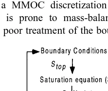
Fig. 6 shows a simplified schematic of the algorithm. The algorithm follows closely those proposed by Chen et al.24 and Vassilev (A. Vassilev, personal communication, 1996). The boundary condition algorithm described above is
particular for the combination of a known flux in the water phase and a known pressure in the air phase. The algorithm is not directly applicable to other combinations of phase fluxes/pressures at the boundary. Different algorithms based on similar iterative techniques will need to be developed for these combinations. The requirement for different iterative algorithms for each boundary type will not add to the computational time required to solve the fractional flow equations. However, the complexity of the computer code will be greatly increased in fractional flow codes that are developed to satisfy generalized boundary conditions. This contrasts with the two-pressure approach, where different boundary conditions can be accommodated relatively easily.
3.5 Mass-balance
A mass-balance calculation provides necessary (but not suf-ficient) verification of the validity of the numerical solution. The mass-balance for the two-pressure solution has been described in Celia and Binning.6They showed that mass-balance errors for this numerical scheme are small. In contrast, a MMOC discretization of the fractional flow equations is prone to mass-balance errors. These arise through a poor treatment of the boundary conditions in the Fig. 5. Integral¹
ZSw
Sc fw¹
1 2
dpc dSw
dSwas a function of saturation in the definition of global pressure using the functional forms of Touma and Vauclin43for the case of air and water phases.
Fig. 6. Sequence of computation for solution of the pressure– saturation equations with general boundary conditions. The numbers in the diagram refer to sequence of steps explained in
MMOC. The mass-balance errors inherent in the MMOC have been noted by Healy and Russell.53 Recently, Dahle et al.48have shown how an ELLAM can be used to address the mass-balance errors inherent in the MMOC discretiza-tion of the saturadiscretiza-tion equadiscretiza-tion. The ELLAM was devised by Celia et al.54to provide a rigorous framework for character-istic methods and an improved treatment of boundary conditions.
The finite difference algorithm of Morel-Seytoux and Billica is based on the conservative form of the governing saturation equation (eqn (13)), and as with any implicit centered finite difference approximation of the conservative form of the advection–dispersion equation, it is perfectly mass conservative.
Mass-balance errors have been calculated for all three methods by comparing the mass change in the domain calculated from the saturations with the boundary fluxes, either specified as a boundary condition or calculated from the solution. The results are reported for a number of simulations below.
4 RESULTS
Several problems relevant to applications in hydrology are presented. They consider multi-phase infiltration of water into a porous medium initially filled with air and water. First a simulation is presented where saturations are specified as the boundary conditions and the total flux is known, so it is only necessary to solve the saturation equation. A
comparison is made of the two-pressure approach, and the finite difference and MMOC solutions of the saturation equation. A second problem is then solved where general hydrologic boundary conditions are applied, so the global pressure equation must also be solved in the fractional flow approach. For both problems, material properties are taken
from the measurements of Touma and Vauclin,43 as
presented above.
4.1 Example 1
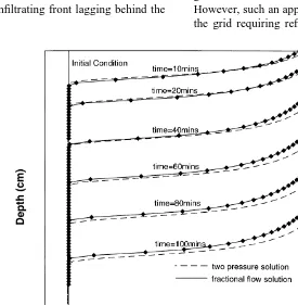
In petroleum engineering applications it is natural to specify boundary conditions in terms of the total flux and the satura-tion of a single fluid. The first example considers a one-dimensional problem in hydrology where it is possible to specify such boundary conditions. For one-dimensional, incompressible flow the pressure equation is degenerate and so the total flux is constant in space and determined by the boundary conditions. If the total flux is specified at the boundary then it is not necessary to solve the pressure equation. The first example considers infiltration of water into an initially dry soil with a uniform normalized satura-tion of 0.1646. The normalized water saturasatura-tion at the soil surface is specified to be 0.9159, and at the bottom of the soil column it is 0.1646. The bottom of the column is sealed to both the air and water phases, so that the total flux is zero. Note that the boundary conditions at the bottom of the column, qw¼qa¼0 and Sw¼0.1646, are over-specified (normally the saturation at the bottom of the column would not be given) to avoid the need for an iterative procedure to
Fig. 7. Solution of a problem with constant saturation boundary conditions using three different numerical methods. The MMOC is shown with nodes marked. The finite difference solution and the two-pressure solution are shown as solid lines and are indistinguishable from each other. The computational effort involved in the MMOC solution is about one tenth that of the other techniques (see Table 1). There is,
determine the bottom boundary conditions. For water to infiltrate into the column it is necessary for the air to escape through the soil surface. This is possible since the soil surface is not saturated.
The problem is solved using three numerical methods. The first is the two-pressure solution. The others are based on the fractional flow approach, and use the MMOC and a finite difference approximation to solve the saturation equation. The two-pressure solution employs a spatial discretization with elements of sizeDz¼1 cm and variable-sized time steps. The total simulated time is 100 min, and the initial time step size isDt¼2 s. Initially it is necessary to employ a small time step as the pressure changes are steep at the infiltrating front and so the nonlinearities are strong. However, as the water infiltrates into the column the infil-trating front smooths, so the nonlinearities weaken and larger time steps can be taken. In this case the time step can be increased from its initial size of 2 s, up to 116 s at the end of the simulation. In each iteration the error tolerance on the residual (See eqns (18) and (19)) is set to be 1310¹3
.
The finite difference solution employs the same spatial grid as the two-pressure solution, and constant sized time steps of sizeDt¼200.0 s. The time step size is chosen to be as large as possible, and is constrained by the need to ensure that the nonlinear iteration scheme is convergent. The error tolerance in the nonlinear iteration scheme on saturation is 0.001.
The MMOC solution employs a coarse spatial grid with Dz¼10.0 cm and localized grid refinement with the same grid size as used in the two-pressure solution. The grid is refined whenever the saturation change between neigh-boring nodes exceeds 0.05 (see the solution in Fig. 7 for a typical grid). A constant sized time step of 600 s is used and the error tolerance on the nonlinear iteration schemes is set to be 0.001 on the saturation.
A comparison of the solutions obtained by the three methods is given in Fig. 7. Table 1 gives a comparison of the computational effort required by the three methods. The results from the three simulations suggest a significant difference in computational efficiency. The two-pressure solution was the most inefficient scheme, the finite difference solution of the saturation equation marginally better, and the MMOC solution of the saturation equation the most efficient solution technique.
The efficiency of the MMOC is due to the lack of restric-tion on time step size. The only restricrestric-tions of time step size
with the MMOC are due to the iteration scheme in the solution of the ‘diffusion correction’ equation with a larger number of iterations required as the strength of the non-linearities increases. The single step integration of the hyperbolic part of the equation will also become more inaccurate with choice of a larger time step size. In contrast, the time step choices for the finite difference and two-pressure solutions are restricted by a Courant number criterion, which for explicit schemes can be given by35
Cr¼1
J
Fw(Stw)¹Fw(Sbw)
St w¹Sbw
! Dt
Dx,1
For the implicit schemes employed here the Courant number criterion is less strict,55,56 but is still a good guide for choice of time step.
4.2 Example 2
In hydrology, boundary conditions are frequently specified in each phase separately. A common problem specifies a flux in the water phase and a pressure in the air phase. In this case the coupled pressure and saturation equations must be solved simultaneously. For the present example, a column of soil is considered with a normalized initial saturation of 0.1655. The boundary conditions for the problem are that the water flux is fixed at 8.3 cm h¹1and the air pressure equal to 0 cm water at the soil surface. The air pressure is set to be 0.1204 cm and the water pressure
¹99.8796 cm at the bottom of the soil column. The air boundary conditions are chosen to be those for a static equilibrium in the air phase and the bottom boundary con-dition on the water phase is chosen to match the initial water content of the column. The column is filled with a coarse sand, having the properties given in Fig. 3. The problem was modeled by Celia and Binning6 using the two-pressure approach. The problem is solved here using both the fractional flow approach and the two-pressure solution and comparisons are made between the methods.
The fractional flow approach employs the MMOC to solve the saturation equation and the finite element method to solve the pressure equation. The iterative methodology described previously is used to determine the boundary con-ditions. A coarse grid of 11 nodes with a spacing of 10 cm is used. The grid is locally refined, with each element being broken into 10 smaller elements whenever the normalized saturation change between neighboring nodes exceeds 0.05.
Table 1. Comparison of the numerical efficiency of techniques for solving the two-phase flow problem in a case with fixed saturation boundaries
Two-pressure solution MMOC Finite difference
Computational time (s) (Sun SPARCstation 5) 43.1 60.0 34.0
Number of time steps 96 10 30
Courant number 0.055–1.06 5.52 1.84
Iterations/time step 3–10 14–2 6–13
This value was chosen as it provides a good balance between computational efficiency and accuracy. Ten time steps of size 10 min are employed in the solution. Error tolerances on each of the iterative processes in the code must also be specified. These are the iterative characteristic solver and the iterative ‘diffusion correction’ in the solution of the saturation equation, and the iteration criteria for con-vergence of the boundary conditions. In all three cases an error tolerance of 1310¹3was specified on the normalized
saturation.
The two-pressure solver uses a grid with the same resolu-tion as the refined grid of the fracresolu-tional flow solver, i.e. 101 nodes of spacing 1 cm. A time step size of 6 s is initially applied, and the time step is increased by a factor of 1.05 at later times when the number of nonlinear iterations falls below 10. Using this time step acceleration scheme the time step size could be increased from the initial 6 s to 101 s at the end of the simulation. The convergence criteria on the solution is 1310¹3on the residual.
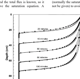
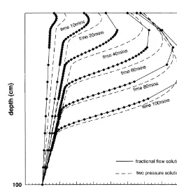
The two solutions are compared in Figs 8 and 9, and the computational cost of each solution is shown in Table 2. Fig. 8 shows saturation as a function of depth at various time intervals. The distribution of nodes used in the fractional flow solution is also shown in the figure. As can be seen from the figure, the fractional flow solver has used a refined grid in the neighborhood of the steep infiltration front. The two-pressure solution is perfectly mass conservative. In contrast the fractional flow solution shows a 4% mass balance error, with the infiltrating front lagging behind the correct location.
Fig. 8 shows that the infiltrating water has a fairly uniform frontal speed and a constant shape. The uniform frontal speed is given by the Buckley–Leverett equation. The infiltrating front retains its shape as the capillary diffu-sion is exactly balanced by the self-sharpening character of the hyperbolic part of the equation. These observations are the key to the computational efficiency of the MMOC solu-tion. Note also that Fig. 3c shows that the capillary diffusion acts only over high ranges of saturation, as observed in Fig. 8. Analysis of the fractional flow function and the capillary diffusion function give a good a priori idea of the form of the solution to the equations.
Fig. 9 shows the global pressure corresponding to the saturation solution shown in Fig. 8. The global pressure is a mathematical convenience and so no physical interpreta-tion can be made of this figure. The figure does show one problem with the fractional flow approach. The localized grid refinement is based on gradients of the normalized saturation and not on the global pressure. As can be seen from Fig. 9 the global pressure gradient is quite large in regions remote from the saturation front. In particular, the global pressure variation at the boundary is quite large. However, the coarse grid is used at the boundary after the infiltration front has moved into deeper parts of the column. This leads to quite large errors in the determination of the boundary conditions. A modified grid refinement algorithm could be employed where both the pressure and saturation gradients are used to determine the degree of refinement. However, such an approach would lead to large portions of the grid requiring refinement, reducing the computational
advantages of localized grid refinement for the example being considered here.
The two-pressure solution is more accurate than the frac-tional flow solution, with large errors in the fracfrac-tional flow solution due to discretization errors leading to a poor treat-ment of the boundary conditions. The computational effort involved in obtaining these solutions is given in Table 2. The two-pressure solution requires about twice as much computational time as the fractional flow solution. The frac-tional flow solution required 31.85 s on a Sun workstation. Of this time the majority was spent in solving the highly nonlinear saturation solution (29.9 s), with only a small amount of time required to solve the much better behaved pressure equation (1.0 s).
The simulation shown here has been chosen to illustrate the deficiencies of the fractional flow solution. As the spatial and temporal discretizations are refined the solutions con-verge. To obtain a solution with the fractional flow approach that is of similar accuracy to the two-pressure solution requires a uniform fine grid. Localized grid refinement based only on the saturation solution does not give satis-factory results. If the fractional flow solution is required to obtain a high accuracy solution the advantages in computa-tional efficiency of the method over the two-pressure approach disappear.
5 DISCUSSION
Numerical solutions based on the fractional flow form of the governing equations appear potentially attractive, because of the relatively simple form of the pressure equation (eqn (11)), and the hyperbolic character of the saturation equation (eqn (13)). Numerical algorithms can be designed to take advantage of these properties, with the aim of gain-ing significant improvements in computational efficiency.
The results presented here show that for problems in one dimension where the saturation equation alone can be solved, the fractional flow approach is far more efficient
than equivalent solvers employing the two-pressure
approach. However, for generalized boundary conditions, such as those frequently employed in hydrology, the full pressure–saturation solution of the fractional flow equations must be coupled with an iterative scheme to find the correct boundary conditions. In this case there was little or no computational advantage gained by the fractional flow approach.
The fractional flow approach, while offering some computational attractions, is also far more complex to understand and to implement in computer codes. The
two-pressure code requires approximately 690 lines of
generously commented code, whereas the fractional flow Fig. 9. Global pressure obtained using the two-pressure and fractional flow approaches for the problem illustrated in Fig. 8.
Table 2. Comparison of computational effort for the fractional flow and two-pressure solutions for the problem illustrated in Fig. 8
Two-pressure solution Finite difference
Computational time (s) (Sun SPARCstation 5) 48.9 31.85
Time steps 105 10
Iterations/time step 5–10 5–19 diffusion, 3–11 boundary
code requires 2080 lines. The largest portion of the frac-tional flow code is the MMOC solution of the saturation equation. Given that no computer code is ever bug free, the significantly larger amount of computer code required for the fractional flow approach should be a serious consideration when choosing the solution methodology.
The results presented here are for one dimension. It is possible that in higher dimensions the fractional flow approach will become more competitive. For example, it was shown in Binning45 that the time step acceleration that can be used very successfully in one dimension with the two-pressure approach, gives little advantage in higher dimensions. In contrast the fractional flow approach has been demonstrated to be equally effective with large time steps for petroleum problems in both one and higher dimen-sions.18Until the time when the higher-dimensional version of the fractional flow approach with general boundary conditions has been completed, no final conclusions on the efficiency of the method can be made.
There are a number of drawbacks to the fractional flow formulation. These include the non-physical nature of the total pressure term; the associated complications in imple-menting boundary conditions whose specification is associated naturally with individual phases instead of combinations of phase information; the complications intro-duced by the nature of the gravity terms; the difficulties in dealing with multiple infiltration and drainage fronts; the problem of including compressibility; and the complications in the characteristic solution when material heterogeneity is introduced.
Implementation of general boundary conditions requires different iteration schemes for each different pair of phase-specific boundary conditions, one example of which is given above. This causes both additional coding and additional computations which largely offset the gains made by developing numerical methods that exploit the form of the
governing equations. Note that for one-dimensional
problems, the analytical techniques of Morel-Seytoux and Billica12,13 can be used to avoid solving the full pressure equation. However, that approach does not generalize easily to multiple dimensions, while the approach presented herein does. The gravity issue has been addressed effectively by Hansen et al.,23 although its implementation in multiple dimensions implies some additional coding.
The two outstanding issues that appear to be most significant at this time are the treatment of material hetero-geneities in which the fractional flow function varies spatially, and the treatment of multiple infiltration and drainage fronts. Earlier work, by for example Langlo and Espedal,21 incorporated heterogeneity in the intrinsic permeability only, with the relative permeabilities (and therefore the fractional flow functions) remaining spatially constant. The more difficult case of heterogeneous fractional flow functions requires that the splitting technique used to determine frontal speeds and the associated numerical characteristic curves must account for underlying variability within a time step. This appears to have
implications for the back-tracking step of the characteristic solution and the treatment of the ‘anti-diffusion’ correction that is associated with the fractional flow splitting. Because numerical solutions are quite sensitive to the treatment of the anti-diffusion, additional study appears to be needed to incorporate general material heterogeneities. A similar situation arises when multiple infiltration and drainage fronts occur, as might be expected for simulation of inter-mittent rainfall events. In this case, different fractional flow splittings are required for the different fronts, even when hysteresis is ignored.
One of the most appealing features of the fractional flow formulation is the physical insight offered by the form of the saturation equation, as recognized by pioneers in this area including Buckley and Leverett10 and Morel-Seytoux.1 While numerical methods based on the fractional flow formulation of the governing equations are very attractive for simple model problems, their extension to practical problems remains to be demonstrated. The results presented here for general boundary conditions suggest that potential gains in numerical performance due to the equation form may be offset by the additional complications of the method. Much work needs to be done before numerical methods based on the fractional flow approach will be able to compete with methods having more general applic-ability, such as those of Celia and Binning6and Forsyth and coworkers.34,35
ACKNOWLEDGEMENTS
This work was supported in part by the U.S. Department of Energy under Grant DE-FG02-95ER25267. We wish to acknowledge the contributions of Richard Ewing, Magne Espedal, and Helge Dahle to this work. We would also like to thank the Journal Editor and the anonymous reviewers for their comments on the paper.
REFERENCES
1. Morel-Seytoux, H.J. Two-Phase flows in porous media.
Advances in Hydroscience, 1973, 9, 119–202.
2. Ewing, R.E., Three-phase flow formulations. In
Computa-tional Methods in Water Resources XI, Vol. 1, ed. A.A.
Aldama, J. Aparicio, C.A. Brebbia, W.G. Gray, I. Herrera and G.F. Pinder. Computational Mechanics Publications, Southampton, 1996.
3. Pinder, G.F. and Abriola, L.M. On the simulation of non-aqueous phase organic compounds in the subsurface. Water
Resources Research, 1986, 22, 109S–119S.
4. Sleep, B.E. and Sykes, J.F. Modeling the transport of volatile organics in variably saturated media. Water Resources
Research, 1989, 25, 81–92.
5. Kaluarachchi, J.J. and Parker, J.C. An efficient finite elements method for modeling multiphase flow. Water
Resources Research, 1989, 25, 43–54.
6. Celia, M.A. and Binning, P. Two-phase unsaturated flow: one dimensional simulation and air phase velocities. Water
7. Binning, P. and Celia, M.A., Coupled air-water flow and contaminant transport in the unsaturated zone: A numerical model. In Shallow Groundwater Systems, ed. P. Dillon and I. Simmers, IAH Int. Contributions to Hydrogeology 18. A.A. Balkema, 1998.
8. Binning, P., Celia, M.A. and Johnson, J.C., Two-phase flow
and contaminant transport in unsaturated soils with applica-tion to low-level radioactive waste disposal. Nuclear
Regulatory Commission, Washington, DC, NUREG/CR-6114 Vol. 2, 1996.
9. Schrefler, B.A. and Xiaoyong, Z. A fully coupled model for water flow and air flow in deformable porous media. Water
Resources Research, 1993, 29, 155–167.
10. Buckley, S.E. and Leverett, M.C. Mechanism of Fluid Displacement in Sands. Trans. AIME, 1942, 146, 107–116. 11. Sander, G.C., Norbury, J. and Weeks, S.W. An exact solution
to the nonlinear diffusion–convection equation for two-phase flow. Quarterly Journal of Mechanics and Applied Mathematics, 1993, 46, 709–727.
12. Morel-Seytoux, H.J. and Billica, J.A. A two-phase numerical model for prediction of infiltration: Applications to a semi-infinite column. Water Resources Research, 1985, 21, 607– 615.
13. Morel-Seytoux, H.J. and Billica, J.A. A two-phase numerical model for prediction of infiltration: Case of an impervious bottom. Water Resources Research, 1985, 21, 1389–1396. 14. Wangen, M. Vertical migration of hydrocarbons modelled
with fractional flow theory. Geophysical Journal International, 1993, 115, 109–131.
15. Chen, Z., Espedal, M. and Ewing, R.E. Continuous-time finite element analysis of multiphase flow in groundwater hydrology. Applications of Mathematics, 1995, 40, 203–226. 16. Douglas, J. Jr Finite difference method for two-phase incompressible flow in porous media. SIAM Journal of
Numerical Analysis, 1983, 20, 681–696.
17. Espedal, M.S. and Ewing, R.E. Characteristic Petrov– Galerkin subdomain methods for two-phase immiscible flow. Computer Methods in Applied Mechanics and Engineering, 1987, 64, 113–135.
18. Dahle, H.K., Espedal, M.S., Ewing, R.E. and Saevareid, O., Characteristic adaptive subdomain methods for reservoir flow problems. Numerical Methods for Partial Differential
Equations, 1990, 6, 279–309.
19. Dahle, H.K., Espedal, M.S. and Saevereid, O. Characteristic, local grid refinement techniques for reservoir flow problems.
International Journal for Numerical Methods in Engineering,
1992, 34, 1051–1069.
20. Celia, M.A. and Binning, P., Multiphase models of unsatu-rated flow: approaches to the governing equations and numerical methods. In Proceedings IX International Conference Computational Methods Water Resourses Vol 2: Mathematical Modeling in Water Resources, ed. T.F. Russell et al. Elsevier Applied Science, London, 1992. 21. Langlo, P. and Espedal, M.S. Macrodispersion for two phase, immiscible flow in porous media. Advances in Water
Resources, 1994, 17, 297–316.
22. Langlo, P. and Espedal, M.S., Heterogeneous reservoir models, two-phase immiscible flow in 2-D. In Computational
methods in Water Resources IX, Vol. 2: Numerical Methods in Water Resources, ed. T.F. Russell, R.E. Ewing, C.A.
Brebbia, W.G. Gray, and G.F. Pinder, Elsevier Applied Science, London, 1992.
23. Hansen, R., Espedal, M.S. and Nygaard, O., An operator splitting technique for two-phase immiscible flow dominated by gravity and capillary forces. In IX International
Con-ference on Computational Methods in Water Resources,
Vol. 1, ed. T.F. Russell, R.E. Ewing, C.A. Brebbia, W.G. Gray, and G.F. Pinder, Elsevier Applied Science, London, 1992.
24. Chen, Z., Ewing, R.E. and Espedal, M., Multiphase flow simulation with various boundary conditions. In
Computa-tional Methods in Water Resources X, Vol. 2, ed. A.
Peters, G. Wittum, B. Herrling, U. Meissner, C.A. Brebbia, W.G. Gray and G.F. Pinder, Kluwer Academic Publishers, Dordrecht, 1994.
25. Ewing, R.E. Simulation of multiphase flows in porous media.
Transport in Porous Media, 1991, 6, 479–499.
26. Ewing, R.E. and Heinemann, R.F., Incorporation of mixed finite elements methods in compositional simulation for reduction of numerical dispersion. Reservoir Simulation
Sym-posium, San Francisco, CA, 1983, Soc. Petrol. Eng., Dallas,
TX, SPE 12267, 1983.
27. Ewing, R.E. and Heinemann, R.F. Mixed finite elements approximations of phase velocities in compositional reservoir simulation. Computer Methods in Applied Mechanics and
Engineering, 1984, 47, 161–175.
28. Guarnaccia, J.F. and Pinder, G.F., NAPL: A mathematical
model for the study of NAPL contamination in granular soils, equation development and simulator documentation.
The University of Vermont, RCGRD #95-22, 1997. 29. Spillette, A.G., Hillestad, J.G. and Stone, H.L., A highly
stable sequential solution approach to reservoir simulation.
Soc. Pet. Eng. 48th Ann. Meet., Las Vegas, NV, SPE Paper
no. 4542, 1973.
30. Faust, C.R. Transport of immiscible fluids within and below the unsaturated zone. Water Resources Research, 1985, 21, 587–596.
31. Kueper, B.H. and Frind, E.O. Two-phase flow in hetero-geneous porous media, 1. Model development.. Water
Resources Research, 1991, 27, 1049–1057.
32. Moridis, G.J. and Reddell, D.L. Secondary water recovery by air injection, 1. The concept and the mathematical and numerical model. Water Resources Research, 1991, 27, 2337–2352.
33. Pruess, K., TOUGH user’s guide. U.S. Nuclear Regulatory Comission, Washington, DC, CR-4645, 1987.
34. Forsyth, P.A. A positivity preserving method for simulation of steam injection for NAPL site remediation. Advances in
Water Resources, 1993, 16, 351–370.
35. Unger, A.J.A., Forsyth, P.A. and Sudicky, E.A. Variable spatial and temporal weighting schemes for use in multi-phase compositional problems. Advances in Water Resources, 1996, 19, 1–27.
36. Abriola, L.M. and Rathfelder, K. Mass balance errors in modelling two-phase immiscible flows: causes and remedies.
Advances in Water Resources, 1993, 16, 223–239.
37. Haverkamp, R. et al. A Comparison of Numerical Simulation Models for One-Dimensional Infiltration. Soil Sci. Soc. Am.
J., 1977, 41, 285–294.
38. Russell, T.F., Modeling of multiphase multicontaminant transport in the subsurface. Reviews of Geophysics, Supplement, 1995, 1035–1047.
39. Sleep, B.E. and Sykes, J.F. Compositional simulation of groundwater contamination by organic compounds, 1. Model development and verification. Water Resources
Research, 1993, 29, 1697–1708.
40. Reeves, H.W. and Abriola, L.M. An iterative compositional model for subsurface multiphase flow. Journal of Contaminant Hydrology, 1994, 15, 249–276.
41. Chavent, G. and Jaffre´, J., Mathematical Models and Finite
Elements for Reservior Simulation. North Holland, Amsterdam, 1986.
42. Young, L.C. A study of spatial approximations for simulating fluid displacements in petroleum reserviors. Computer
Methods in Applied Mechanics and Engineering, 1984, 47,
3–46.
analysis of two-phase infiltration in a partially saturated soil.
Transport in Porous Media, 1986, 1, 27–55.
44. van Genuchten, M.T. A closed form equation for predicting the hydraulic conductivity in soils. Soil Sci. Soc. Am. J., 1980, 44, 892–898.
45. Binning, P., Modeling unsaturated zone flow and contami-nant transport in the air and water phases, Ph.D. Thesis, Department of Civil Engineering and Operations Research, Princeton University, 1994.
46. Stothoff, S.A. and Dougherty, D.E., Implementing a three-dimensional two-phase flow model on the connection machine. in Computational Methods in Water Resources
IX, Vol. 1, ed. T.F. Russell, R.E. Ewing, C.A. Brebbia,
W.G. Gray and G.F. Pinder, Elsevier Applied Science, London, 1992.
47. Hansen, R., On the numerical solution of nonlinear reservoir flow models with gravity. Dr. Scient. Thesis, Department of Mathematics, University of Bergen, 1993.
48. Dahle, H.K., Ewing, R.E. and Russell, T.F. Eulerian– Lagrangian localized adjoint methods for a nonlinear advection–diffusion equation. Computer Methods in Applied
Mechanics and Engineering, 1995, 122, 223–250.
49. Welge, H.J. A simplified method for computing oil recovery by gas or water drive. Petroleum Transactions AIME, 1952, 195, 91–98.
50. Dahle, H.K., Adaptive characteristic operator splitting tech-niques for convective-dominated diffusion problems in one and two space dimensions. Thesis, University of Bergen, Department of Applied Mathematics, 1988.
51. Milly, P.C.D. A mass-conservative proceedure for time step-ping in models of unsaturated flow. Advances in Water
Resources, 1985, 8, 32–36.
52. Press, W.H., Flannery, B.P., Teukolsky, S.A. and Vetterling, W.T. Numerical Recipes in C. Cambridge University Press, Cambridge, 1988.
53. Healy, R.W. and Russell, T.F. A finite volume Eulerian– Lagrangian localized adjoint method for the solution of the advection–diffusion equation. Water Resources Research, 1993, 29, 2399–2413.
54. Celia, M.A. et al. An Eulerian–Lagrangian localized adjoint method for the advection–diffusion equation. Advances in
Water Resources, 1990, 13, 187–206.
55. Daus, A.D., Frind, E.O. and Sudicky, E.A. Comparative error analysis in finite element formulations of the advection– dispersion equation. Advances in Water Resources, 1985, 8, 86–95.