Directory UMM :Data Elmu:jurnal:E:Energy Economics:Vol22.Issue4.2000:

(1)

Forecasting energy consumption and energy

related CO emissions in Greece:

₂

An evaluation of the consequences of the

Community Support Framework II and

natural gas penetration

Nicos M. Christodoulakis

a,U

, Sarantis C. Kalyvitis

b

_,

Dimitrios P. Lalas

c

_{, Stylianos Pesmajoglou}

c

a

Department of International and European Economic Studies, Athens Uni¨ersity of Economics and Business, and CEPR, Patission Str. 76, Athens 10434, Greece

b

Athens Uni¨ersity of Economics and Business, Athens, Greece c

National Obser¨atory of Athens, Athens, Greece

Abstract

This study seeks to assess the future demand for energy and the trajectory of CO2

emissions level in Greece, taking into account the impact of the Community Support

Ž .

Framework CSF II on the development process and the penetration of natural gas, which is one of the major CSF II interventions, in the energy system. Demand equations for each

Ž .

sector of economic activity traded, non-traded, public and agricultural sector and for each

Ž .

type of energy oil, electricity and solid fuels are derived. The energy system is integrated into a fully developed macroeconometric model, so that all interactions between energy, prices and production factors are properly taken into account. Energy CO forecasts are2

then derived based on alternative scenarios for the prospects of the Greek economy. According to the main findings of the paper the growth pattern of forecast total energy consumption closely follows that of forecast output showing no signs of decoupling. As regards CO emissions, they are expected to increase with an annual average rate, which is2

JEL classifications:O10; O40; Q43

Keywords:Energy demand; Carbon dioxide emissions; CSF intervention; Natural gas

U

Corresponding author. Tel.:q30-1-8203273; fax:q30-1-8221011.

Ž .

E-mail address:nchris@hermes.aueb.gr N.M. Christodoulakis .

Ž .

(2)

1. Introduction

The importance of energy as a key factor in explaining long-run trends in economic output growth was } to a large extent } neglected until the first oil price shock in 1973. At that time, it became evident that the slowdown in growth and productivity observed in all industrialised countries was closely associated with developments in the energy sector. The investigation of the macroeconomic links, which were revealed then, between energy and the rest of the economy has since offered much scope for economists and policy makers to explain the growth process.

Lately, economic growth and energy consumption are also closely related to environmental considerations, because of concern caused by evidence of anthro-pogenic influence on climate, resulting in the international treaties signed in

Ž . Ž . Ž .

Toronto 1988 , Rio de Janeiro 1992 and Kyoto 1997 controlling atmospheric gases.

In particular, special attention is starting to be paid to the decrease of carbon

Ž .

dioxide CO₂ and other ‘greenhouse’ gases emissions that primarily arise from the

Ž .

consumption of energy. The Council of Ministers of the European Union EU decided in October 1990 that CO emissions should be stabilised by 2000 at the2 level of 1990.1 _{Convinced of the necessity of further action on this matter, the} world community adopted, in December 1997, the Kyoto Protocol to the United

Ž .

Nations Framework Convention on Climate Change UNFCCC . The Kyoto Proto-col sets out further commitments of the developed country Parties of the UNFCCC for the period 2008]2012. The overall target agreed is a reduction of the aggregate

Ž . Ž .

anthropogenic emissions of carbon dioxide CO , methane CH , nitrous oxide₂ ₄ ŽN O , hydrofluorocarbons HFCs , perfluorocarbons PFCs and sulphur hexafluo-₂ . Ž . Ž .

Ž .

ride SF by at least 5% below the 1990 levels for the period 2008₆ ]2012.

The Protocol also sets out a differentiated approach for the achievement of such a reduction target among the Parties involved. Under the provisions of Article 4 of the Protocol that enables the joint fulfilment of the commitments undertaken, the

Ž .

overall target for the EU y8% will be achieved by an equitable burden sharing between EU member states. The burden sharing should take into account differ-ences in the starting point, national circumstances and historic responsibility of each member state in the occurrence of the ‘greenhouse’ effect. Negotiations amongst EU member states were finalised during the Environment Council in June 1998 and the burden sharing agreement specifies that Greece will have to restrict the average growth of the emissions of all six gases, for the period 2008]2012, to

1 _Ž _{. Ž .}

The decision was prompted among others, by the following factors see Surrey, 1992 : a the

Ž .

consequent action of other policy measures e.g. traffic jams , which are related to the energy

Ž . Ž .

consumption and which have to in any case be enforced ‘no regrets’ policy ; b the wide differences

Ž .

among interested countries, which call for common policy measures; c the necessity of switching to a more efficient use of energy sources, given the inability of substitution with other less pollutive ones;

Ž .

(3)

q25% compared to 1990 levels. This level of ambition will be achieved through a Ž

number of interventions national and EU common and co-ordinated policies and .

measures in all sectors of the economy, and particularly in the energy sector. In this context, the purpose of this work is to provide estimates of energy consumption in Greece by sector of economic activity and by type of energy form. Next, based on these estimates forecasts of the demand for energy will be generated for the period up to 2012, assuming a number of alternative scenarios for the prospects of the Greek economy. The forecasts of energy consumption are then used to derive CO emissions levels, which are closely related to economic₂ growth and energy consumption. Also, attention is focused on the changes in energy consumption and CO emissions brought about by the Community Support₂

Ž . Ž .

Framework CSF II. The CSF II also known as Delors’ II Package is an intervention plan deemed necessary in order to assist the less developed members

Ž .

of the European Union Greece, Spain, Portugal, Ireland to modernise their economies, foster growth and approach the welfare and efficiency of its most developed members. Its second phase, CSF II, which is operational during 1994]1999, is substantially more extensive in actions and far-reaching in impact

Ž .

than the first CSF phase CSF I implemented in 1989]1993, and is expected to have a significant impact on the growth process in these countries.

One of the major CSF II interventions in Greece is the introduction of natural

Ž .

gas NG to the Greek energy system. The actual cost for the NG penetration is estimated at 2 billion ECU and is largely financed by the European Investment

Ž .

Bank. According to the works programme of Public Gas Corporation PGC , total absorption of NG will reach 3.5 billion Nm3 _{per year by 2005.}2 _{An extended} infrastructure system has been designed and is now near completion in order to carry imported NG to the main consumption areas: first, in the electricity genera-tion sector and large industrial units and, next, in the residential and commercial sectors } though at slower rates.3

To enable the analysis of the above effects, it is better to integrate the demand and supply of energy into a full-developed macroeconomic model, so that price]quantity interactions are properly taken into account. Therefore, we employ a sectoral macroeconometric model of Greece and after estimating demand

2

Approximately 85% of this total will be imported from Russia, via Bulgaria, by pipeline and the remaining 15% will be imported from Algeria in liquefied form. The construction of the main transmission pipeline was completed in July 1995, while the construction of secondary pipelines is

Ž .

progressing. The supply of natural gas to the first Public Power Corporation PPC gas-fired power station began in 1997, while two more power stations in South Attica are scheduled to come on-line by the end of 1998. Furthermore, another natural gas fired station in northern Greece is expected to come on-line by the end of 2001. According to the specified timetable, it is estimated that the PPC will be in a position to absorb approximately 1.1 billion Nm3_{of natural gas by the year 2000 and 1.5 billion Nm}3_by

the year 2001.

3

In the industrial sector, PGC has already formulated a pricing policy and the general terms of gas supply to industrial customers, and is aggressively pursuing contracts with industrial customers. Nine contracts have already been signed for more than 0.3 billion Nm3_r_{year and a few large industrial units}

(4)

functions by sector of economic activity and type of energy, the whole model is used to forecast how these variables are likely to develop in the medium-term.

In a related macroeconomic study without including energy modelling,

Christo-Ž .

doulakis and Kalyvitis 1998a analysed a number of scenarios for the growth patterns of Greece for the period up to the year 2010. The same authors ŽChristodoulakis and Kalyvitis, 1997 analysed the macroeconomic aspects of CSF. II effects on energy demand in Greece, but without including the introduction of NG. The present paper extends this work, first, by explicitly including the penetra-tion of NG, in conjuncpenetra-tion with CSF effects in the energy system, second, by employing more powerful econometric modelling techniques to the key equations of the energy model, third, by using an updated data set covering the period 1974]1994 and extending the time horizon to 2012 and, fourth, by computing expected CO emissions in view of the energy demand forecasts.2

In particular, the forecasting exercise takes place under alternative assumptions about the effects that CSF II is likely to have on the Greek economy. First, a benchmark forecast presenting economic developments in the absence of CSF interventions and NG penetration in the energy system is examined. Next, a case is examined based on the benchmark forecast but with the assumption that NG introduction satisfies additional electricity demand. Finally, two scenarios that take into account the impact of total CSF actions without and with NG penetration, respectively, on energy consumption and CO emissions are examined.₂

In Section 2 of the paper, the structure of energy system and the estimation

Ž .

equations are discussed and presented and are given analytically in Appendix A together with the procedure for calculating the related CO emissions. In Section2 3, the four scenarios for the derivation of forecasts of final energy demand and CO emissions in Greece until the year 2012 are described. In Section 4 we assess₂ the quantitative effects under these scenarios on energy consumption and CO₂ emissions, and, finally, in Section 5 the main conclusions are presented.

2. Modelling energy consumption in Greece

To capture the effects of energy on the productive side of the economy, we consider the demand for energy by each sector of the economy. The production

Ž .

bloc consists of three aggregate sectors: a the tradable sector that includes Ž .

manufacturing and mining; b the non-tradable sector that includes transport and

Ž . 4

commercial activities; and c the aggregation of public and agricultural sectors.

Ž .

Following the approach adopted by Christodoulakis and Kalyvitis 1997 , the distinction is made in order to conform with the annual four-sector

macroecono-Ž .

metric model for Greece described in Christodoulakis and Kalyvitis 1998a to which the present demand system will be incorporated for forecasting and simula-tion analysis.

Ž

As regards final energy demand by type of energy used Oil, Electricity and .

(5)

activity for the period 1974]1994: the industrial sector, the transport sector and the housingrcommercial sector. Using this classification, the various types of energy

Ž . Ž .

are grouped in three main categories: i Oil liquid fuels including petrol consumed by industry, gasoline, diesel and fuel oil consumed by the transport

Ž .

sector and heating-oil used by the housing and commercial sectors; ii Electricity Ž . consumed by industry, transport, housing and commercial sectors; and iii Coal Žsolid fuels that include all solid sources of energy consumed by industry..

Since data published for the commercial, housing and transport sectors include energy used aggregately by the non-tradable sector and the public and agricultural sectors taken together, demand for energy in each of those categories is obtained proportionally to the output share of those sectors:

Ž

v Energy demand by non-tradable sectors Total energy demandyEnergy demand

.U_Ž _Ž

by tradable sector Non-tradable sector outputr Total outputyTradable sector ..

output

Ž

v Energy demand by public and agricultural sectorss Total energy demandy Energy demand by tradable and non-tradable sectors

Ž .

Demand for solid fuel that amounts to approx. 5% of total energy consumption is not modelled behaviourally but serves as a residual between total energy demanded by the three sectors and the demand for the two previously estimated types of energy. The residual equation is:

v Demand for solid fuelsEnergy demand in tradable, non-tradable, public and agricultural sectorsyDemand for oil and electricity

Energy demanded by each production sector is a function of sectoral output and Ž .

the real price of energy in each sector where: i for the tradable sector, the real price of energy is the ratio of energy price in industry to tradable sector output

Ž .

deflator; and ii for the non-tradable and public-agricultural sectors, the real price of energy is defined as the ratio of an expenditure-weighted price index of energy in the transport, housing and commercial sectors relative to non-tradable sector

4

Annual energy data on quantities and prices are provided by the Ministry for Development for the period 1974]1994. Quantities of energy consumed by sector are divided in the following three categories in accordance with the classification in the Annual Energy Balances, issued by the Ministry for Development: A. Industry: Consumption of the extractive industries, manufacturing and construc-tion. B. Transportation: Consumption for transportation irrespective of transport means, excluding consumption for international sea transport and including energy consumption for all air-transport activities. C. HousingrCommercial: Consumption of households, commercial establishments, services, agriculture, etc. Quantities by type of energy are divided in the following three categories in accordance with the classification in the Annual Energy Balances, issued by the Ministry for Development: A.Solid

Ž . Ž .

(6)

Table 1

Energy model: the structure of behavioural equations

Energy demand by sector

Ž .

Tradable sectorsf tradable sector output, real price of energy in the tradable sector

Ž .

Non-tradable sectorsf non-tradable sector output, real price of energy in the non-tradable sector

Ž .

Public-agricultural sectorsf public-agriculture sector output

Energy demand by type

Ž .

Oilsf total output, real price of oil

Ž .

Electricitysf total output, real price of electricity

Energy prices

Ž .

Tradable sectorsf price of oil, price of electricity, price of solid fuel

Ž .

Non-tradable sectorsf price of oil, price of electricity

Price linkages

Ž .

Tradable sector deflatorsf nominal unit labour cost, imports deflator, weighted energy price index

Ž .

Non-tradable sector deflatorsf nominal unit labour cost, weighted energy price index

Ž .

Wholesale price indexsf nominal unit labour cost, imports deflator, weighted energy price index

output deflator.5 _{Demand equations for the various types of energy are modelled} as functions of the associated price indices relative to GDP deflator and using total output as a measure of activity.6 _{Own-price coefficients are expected to be negative} while positive activity coefficients indicate a ‘luxury’ type of energy that rises with output and negative ones characterise a ‘necessity’ type of energy. The structure of the behavioural equations of the energy model is given in Table 1.7

Turning to the equations for sectoral demand of energy, one observes that the

Ž .

long-run output elasticities reported in Table 2 are 0.76, 1.51 and 1.95 for the tradable, non-tradable and public-agricultural sectors, respectively, while the corre-sponding short-run elasticities are 0.79, 1.27 and 0.64. As regards the price elasticities, they are found to bey0.19 andy0.24 in the long-run for the tradable and non-tradable sectors, respectively, while in the short-run they are found to be y0.25 and y0.23, respectively. The demand for energy by the public-agricultural sector appears to be insensitive to changes in real prices, probably because of the lower substitution possibilities with other production factors in these sectors of economic activity.

5 _Ž _.

This specification i.e. with real prices and sectoral output as independent variables could be derived by factor demand equations based on a production function with energy as an input. However, given the complex non-linear relationships postulated by such a scheme, estimation via the error-correc-tion specificaerror-correc-tion would be inappropriate, and thus, we opted for this }more flexible }functional form.

6 _Ž _.

For a description of this approach see Boone et al. 1992 .

7 _Ž

Since all of the series at hand are found to be non-stationary see Christodoulakis and Kalyvitis,

. Ž .

(7)

Table 2

a

Estimated elasticities of energy demand with respect to output and prices

Energy demand Output Price

Long-run Short-run Long-run Short-run

Tradable sector 0.76 0.79 y0.19 y0.25

Non-tradable sector 1.51 1.27 y0.24 y0.23

Public-agricultural 1.95 0.64 ] ]

sectors

Oil 1.00 0.78 y0.22 y0.16

Electricity 1.76 1.12 ] y0.14

a

Elasticities of sectoral energy demand are with respect to sectoral output and sectoral real prices while elasticities of type of energy demand are with respect to total output and total real prices.

The demand for oil has an output elasticity of 1.0 in the long-run, while the demand for electricity has a long-run output elasticity of 1.76. The short-run output

Ž .

elasticities are smaller 0.78 and 1.12, respectively . The own-price elasticities for

Ž .

oil is rather small y0.22 andy0.16 in the long- and short-run, respectively while the own-price elasticity for electricity is y0.14 in the short-run; the long-run elasticity is found statistically insignificant and is omitted from the long-run equation. Finally, the demand for electricity adjusts slower to its long-run

equilib-Ž

rium relationship the adjustment parameter isy0.23 while that of oil demand is

.8

y0.51 .

Energy prices are modelled with homogeneity of degree one imposed and accepted by the data. The domestic prices of energy components are modelled as functions of the domestic unit labour cost and the price of imported oil, which is equal to the price of crude oil in USDrbarrel9 _{multiplied by the Drachma}

rUSD

exchange rate. To account for the effect of taxes on domestic oil prices, the latter are adjusted by the average Value Added Tax rate.10

The results show the serious dependence of domestic oil prices on the external component; the price of oil is found to depend by 40% on the foreign price of oil

Ž .11

while the latter explains only a small fraction of the price of electricity 4% . The aggregate price indices used for energy demand in the tradable and non-tradable

8 _Ž _.

The results are similar with findings by Donatos and Mergos 1989 who use data for the period 1963]1984 and estimate the demand for energy as a function of prices and income. The authors find that ‘energy demand declines with an increase in unit prices and increases with income’ and that ‘energy demand is price inelastic while the demand for liquid fuels is income elastic’.

9

The oil price considered here was taken as the average crude price derived from spot crude oil prices for Dubai, UK Brent and Alaskan N. Slope reserves, which correspond to equal consumption of medium light and heavy oil on a world-wide scale.

10

A dummy is included for the year 1986 in the price of oil equation when the international price of oil fell by 60%, but the fall is not directly transmitted to domestic oil prices due to administrative controls.

11

(8)

sectors are modelled as convex weighted averages of the corresponding prices of the three types.

Finally, we have to model the effects of energy prices on the price mechanism of the annual macroeconometric model. The basic price equations in the macro model are modified so as to include an energy price composite index together with unit labour cost and the price of imports.12 _{The composite price index is calculated} as the sum of the products of the weights in final demand of each type of energy and the corresponding price. These three prices drive the remaining prices in the model. The results suggest that the wholesale price index depends by 55% on domestic unit labour cost, 18% on the price of imports, while the remaining 27% is due to the price of energy. The corresponding energy burden for the tradable and non-tradable output deflators are only 13% and 16%, respectively.

The system is interacting with a number of macroeconomic variables that are determined in the four-sector econometric model. The linkages operate mainly through two channels: first, through sectoral output which affects the demand for energy in each sector and total output which affects the type of energy demand and, second, through the price mechanism which is affected by energy prices and, in turn, transmits the change in prices in the economy through sectoral deflators

Ž .

and the wholesale price index see also Christodoulakis and Kalyvitis, 1997 .

3. Four scenarios for future energy consumption and its environmental impact

In general, CO emissions from the energy sector are directly related to fuel mix,₂ combustion efficiency and technologies applied. In Greece, energy related activities Žincluding extraction, distribution and combustion of fossil fuels are responsible. for approximately 76% of total national greenhouse gases emitted each year. During 1990]1995, CO emissions from the energy sector accounted for approxi-₂ mately 90% of total CO emissions in Greece, thus making this gas the largest₂ contributor to the so-called ‘greenhouse’ effect.

CO₂ emissions for the period 1995]2012 are calculated by using weighted emission factors for oil, coal and NG disaggregated to the three economic sectors. The emission factors used correspond to aggregate values for the year 1995 and are summarised in Table 3.13 _{In Greece, electricity is predominantly produced by the}

Ž .

combustion of brown coal lignite , heavy fuel oil and diesel oil. Smaller amounts

Ž .

are also produced from renewable energy sources RES which involve mostly hydropower and wind power installations and account for approximately 5% of

12 _Ž _.

Since data for non-fuel import prices are not available, a rise in foreign fuel oil prices operates through two channels: first, by raising the price of imports, and, second, by increasing the domestic price of oil.

13

(9)

Table 3

a

Ž .

Emission factors in kt CO2rktoe for oil, coal and NG aggregated by economic sector

Fuel type Tradable Non-tradable Public-agricultural

Oil 3.17 2.74 3.17

Coal 4.20 n.a. n.a.

NG 2.00 n.a. 2.00

a

n.a., Not applicable.

total electricity production. The calculation of emissions from the use of electricity takes into account the losses incurred during the transformation process at power plants brought about by changes in the average thermal efficiency over the period 1995]2012. The ‘future anticipated’ average thermal efficiency is estimated by considering the fuel mix for each of the four scenarios. Total CO emissions from₂ the electricity production sector are calculated by applying appropriate emission factors for the different fuels used. These factors derive from the approved IPCC ŽIntergovernmental Panel on Climate Change methodology for the completion of.

Ž

inventories of national greenhouse gases see National In¨entory of Greenhouse and .

Other Gases for the years 1990]1995, 1997 .

In this work, we focus on scenarios that incorporate the two main features of interest: the group of actions and initiatives incorporated and co-financed by CSF II and the pivotal role of the introduction of NG in the energy sector. Thus, besides the Benchmarkscenario, which reflects the absence of any new initiatives

Ž

of any kind and in that respect cannot be considered to be a business-as-usual .

scenario , three other scenarios are considered that differ from the benchmark by incorporating the planned use of NG and the CSF II effects first separately ŽBenchmark with NG andCSF II,respectively and then jointly. ŽCSF II with NG..

3.1. Scenario I: Benchmark

The increase in electricity demand is primarily satisfied by the introduction of

Ž .

new lignite and steam coal power units in the interconnected mainland electricity distribution network. At the same time, electric utilities also invest in the area of RES, which are incorporated in the production system of islands to meet increasing power demand in the domestic and tertiary sector. The relative contribution of these systems to total electricity production increases in 2012 to approximately 10.2%. The installation of new, more efficient, thermal units and additional

Ž .

interventions in older units maintenance, combustion efficiency improvements will result in an increase of the average overall thermal efficiency from 34% in 1995 to 36% in the period 2000]2012.

3.2. Scenario II: Benchmark with NG

(10)

electricity demand will be solely satisfied by the introduction of new gas-fired stations in the interconnected distribution network. The effect of the NG penetra-tion to the average thermal efficiency for the period 2000]2012 is an increase to approximately 37%. At the same time, increased emphasis on RES penetration brings their relative contribution to 10.7%.

3.3. Scenario III: CSF II

To capture the impact of CSF II on the Greek economy, we discriminate between two types of effects:

1. demand-side effects, stemming from the rise in private investment and private sector financial wealth, and the substitution of expenditures financed by domestic resources with external transfers;

2. supply-side effects, stemming from the rise in the productivity capacity of firms due to the positive impact that improved infrastructure, more intensive capital formation and an upgraded labour force are expected to have on productivity growth.14

Part of these effects are due to CSF II interventions involving the energy sector per se through a number of projects related to energy production and energy saving, including the development of efficient production methods from RES, the improvement of conventional thermal generation techniques based on lignite, and the installation of emission-reducing equipment.15 _{Under this scenario, total} out-put in the year 2010 is higher than baseline by an impressive 5.9% and, more importantly, output growth rate is above baseline rate by 0.4 percentage units on average.16

The increase in electricity demand is satisfied by the introduction of new gas,

Ž .

lignite and steam coal power units in the interconnected mainland electricity distribution network. The relative contribution of RES systems to total electricity production increases in 2012 to approximately 10%. The average overall thermal efficiency from 34% in 1995 increases to 38% in the period 2000]2012.

3.4. Scenario IV: CSF II with NG

Similarly to Benchmark with NGscenario, under CSF II with NGscenario, after

14

The demand and supply-effects and the calibration and treatment of the aggregate externalities is

Ž .

described in detail in Christodoulakis and Kalyvitis 1998b .

15

In the present context, specific supply-side externalities brought about by energy projects are assumed to be part of the effects generated indirectlythrough total CSF by the combination of hard infrastructure, soft infrastructure, the rise in productive investment and the upgrading of human resources. The objectives of these projects aim first at reducing the dependence on a single energy supply source, improving efficiency of production, increasing availability of alternative energy sources and eliminating shortages, and, second, improving environmental standards, by reducing CO emissions2

and increasing the rational use of more environment-friendly resources.

16 _Ž _.

(11)

2000 all additional electricity demand is solely satisfied by the introduction of new gas-fired stations in the interconnected distribution network, which absorb approxi-mately 3.3 billion m3 _{by the year 2012. The average thermal efficiency for the} target period increases to approximately 39% and the contribution of RES reaches approximately 10%. In addition, there is also a partial substitution of liquid fuels with NG in the tradable and public-tertiary sectors. The gradual penetration of NG into these sectors results in a final consumption of 860 ktoe, or equivalently 1 billion m3 _{of NG by the year 2012. Although, this figure is smaller than the one}

Ž .

expected by the PGC for the same period PNGC, 1997 , it is estimated that the penetration of NG into the domestic and tertiary sector will be rather slow due to inertia in the consumption of households and increased demand needs of gas by

Ž 3 3

the electricity production sector 3.3 billion m compared to 1.5 billion m , which .

also incorporates investment in CHP units by the industry sector .

4. Quantitative evaluation of the four scenarios

In this section we present the projections computed by the model equations based on the four scenarios described in the previous section. To obtain these projections, the same assumptions for the Greek economy described in

Christodou-Ž .

lakis and Kalyvitis 1998a have been adopted. No other constant adjustment of endogenous variables to bring them closer to externally discernible values has been

Ž

made. For the two exogenous variables of the energy model the international price

. Ž .

of oil and the price of solid fuel the following two assumptions are adopted: i the Ž .

international price of oil is assumed to remain constant; ii the price of solid fuel is assumed to continue to grow at the same average rate that prevailed for the estimation period. The benchmark solution is obtained through a dynamic simula-tion of the model over the period 1995]2012, keeping single-equation errors at zero levels.

The forecasts of the model compare well with actual annual energy consumption Ž

provided by the Ministry for Development for the years 1995 and 1996 see Table .

4 . As expected the Benchmark scenario underestimates total energy demand, Ž

while the absolute discrepancy in the CSF II scenario which incorporates the .

cumulative effects of CSF II actions does not exceed 0.3%. These discrepancies are well within the uncertainty range of the actual data collection system and are expressed as ‘statistical differences’ in Annual Energy Balances.

Table 5 displays the model forecasts in terms of energy demand for the Benchmark set of assumptions up to the year 2012. In absolute terms, total final energy demand will reach 24.6 Mtoe at year 2012 from 13.7 Mtoe at year 1990, while the average annual growth rate for the period 1990]2012 is 2.7% p.a. The demand for energy in the tradable sector increases by an average 2.5% p.a., while the corresponding energy demand by the non-tradable sector increases by 3.7%

Ž .

(12)

Table 4

a

Ž .

Comparison between model forecasts and actual fuel consumption in Mtoe for years 1995 and 1996

Oil Electricity Total

Year: 1995

Actual 10.8 2.9 14.7

Ž . Ž . Ž .

Benchmark 10.8 0.6% 2.9 0.0% 14.7 y0.4%

Ž . Ž . Ž .

CSF II 11.0 2.2% 3.0 2.2% 14.6 y0.3%

Year: 1996

Actual 11.6 3.1 15.6

Ž . Ž . Ž .

Benchmark 11.1 y4.0% 3.0 y1.9% 15.3 y1.9%

Ž . Ž . Ž .

CSF II 11.3 y2.5% 3.1 2.1% 15.6 0.3%

a

Numbers in brackets are % deviations from actual consumption.

non-tradable sector in the Benchmark scenario reflect faster growth of non-trad-able output relative to tradnon-trad-able sector output. During the same time period, the demand by the public-agricultural sector will increase by 0.8% per year.

Turning to the demand for each energy type we observe that oil needs decrease over time relative to the demand for electricity; the former increase by 2.1% per year on average, thus reaching 69.8% of total final consumption at year 2012, while electricity demand increases by 2.8% and reaches 21.4% of total final consumption in 2012. The relative contributions of these two fuels for the year 1990 were 74.1% and 17.9% for oil and electricity, respectively, resulting in a fall of the proportion of oil to electricity consumption from 4.1 in 1990 to 3.3 in 2012. Again, these findings confirm previous evidence reported by Christodoulakis and Kalyvitis Ž_{1997 who found that the demand for oil increases relatively slower to that of}. electricity.

Next, using the Benchmark scenario forecasts for demand of oil, electricity and coal of Table 5, and the corresponding emission factors reported in Section 3, CO2

Table 5

a

Ž .

Forecasts of energy demand in Mtoe for the Benchmarkand Benchmark with NGscenarios Variable 1990 1995 2000 2005 2008 2010 2012 Average 1990]2012

2008]2012 % changeryear

TFC 13.7 14.6 17.4 20.1 21.8 23.2 24.6 23.2 2.7

Tradable sector 4.0 4.1 5.2 5.9 6.3 6.6 6.9 6.6 2.5

Non-tradable sector 5.8 6.1 7.4 9.3 10.7 11.7 12.9 11.8 3.7

Public-agricultural 4.0 4.4 4.9 4.9 4.9 4.8 4.8 4.9 0.8

sectors

Oil 10.2 10.8 12.3 14.1 15.3 16.2 17.2 16.3 2.1

Electricity 2.4 2.9 3.4 4.1 4.6 4.9 5.3 5.0 2.8

a

(13)

Table 6

Ž .

Forecasts of CO emissions in Mt and relevant indicators for the₂ Benchmarkand Benchmark with NG a

scenarios

Variable 1990 1995 2000 2005 2008 2010 2012 Average 1990]2012 2008]2012 % changeryear

Benchmark scenario

Total CO2 76.4 81.6 91.5 103.2 111.4 116.5 123.6 117.1 2.2

CO2rGDP 0.158 0.157 0.160 0.163 0.165 0.166 0.169 0.167 0.3

CO2rcapita 7.6 7.8 8.7 9.7 10.4 10.8 11.4 10.9 1.9

Benchmark with NG scenario

Total CO2 76.4 81.6 90.4 98.9 104.4 108.7 113.3 108.8 1.8

CO2rGDP 0.158 0.157 0.158 0.156 0.155 0.155 0.155 0.155 y0.1

CO2rcapita 7.6 7.8 8.6 9.3 9.8 10.1 10.5 10.1 1.5

a

The CO2rGDP indicator is in units of t CO2r1970 thousand DRS and the CO2rcapita indicator is in units of t CO2rinhabitant.

emissions for the period 1995]2012 are calculated and presented in Table 6. For the period 1990]2012, CO emissions are found to increase by an average annual₂

Ž growth rate of approximately 2.2%, thus amounting to an average of 117.1 Mt or

.

an average increase of 53% for the 5-year target period 2008]2012 compared to the 1990 levels. During the target period 2008]2012, the bulk of these emissions

Ž .

are attributed to electricity production 53% , while contributions of the other sectors amount to 15% for the tradable sector, 21% for the non-tradable sector and 11% for the public and tertiary sectors. In absolute values, CO emissions per₂ GDP in constant 1970 prices remain relatively constant compared to CO emis-2 sions per capita for the same time period. By 2012, the former indicator increases

Ž .

by approximately 7% or at an average annual growth rate of 0.3% , whilst the latter follows closely the growth rate of total CO emissions, mainly due to the2 modest projected population increase, which is estimated to approximately 6.5% in total from 1990 to 2012.

As displayed in the second part of Table 6, the introduction of NG in the electricity production sector has a marked effect on total CO2 emissions for

Ž .

Greece Benchmark with NG scenario . This can be attributed to both the lower Ž

carbon content of gas 0.6 tCrMtoe compared to indicative values of 1.4 tCrMtoe .

for lignite and 0.8 tCrMtoe for oil and the improved overall thermal efficiency of electricity production stations. For the target period, average annual total CO₂ emissions amount to 108.8 Mt, or 42% above 1990 levels, compared to 53% for the Benchmark scenario. This increase results in an annual growth rate of

approxi-Ž .

(14)

As shown in Table 7 and Fig. 1, results change considerably when the effects of

Ž .

CSF II actions are included CSF II scenario . Total energy consumption will be higher by 10.4% on average for the target period 2008]2012 compared to the Benchmark scenario, while the annual average growth rate of energy demand for the period 1990]2012 is above baseline by approximately 0.5 percentage units amounting to 3.2% per year. The demand for oil will be higher by 7.7%, and the demand for electricity by 11.0% in year 2012. On average, demand for electricity is higher by 11.3% per year for the period 2008]2012 while the demand for oil increases by 7.6% per year, compared to the Benchmark scenario. Thus, as in

Ž .

Christodoulakis and Kalyvitis 1997 , CSF intervention causes a rise in the relative share of the demand for electricity. Following the significant rise of output, particularly during the CSF implementation period 1994]1999, energy demand by the tradable sector increases with an annual average growth of 2.0% over the period 1990]2012, while the corresponding energy needs of the non-tradable sector and of the public-agricultural sectors increase by 5.0% and 1.4%, respectively, relative to Benchmarkscenario.

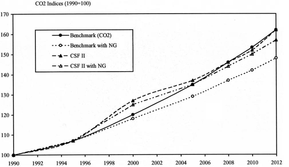
As before, resulting CO emissions are calculated by using the estimated energy2 demand forecasts, shown in Table 7, and the corresponding emission factors. The results for CSF II and CSF II with NG scenarios are presented in Table 8 and a comparison with the other two scenarios is illustrated in Fig. 2. Up to the year 2000, CO emissions are expected to increase almost linearly at an average annual₂ growth rate of approximately 2.3%. After 2000, however, there is a marked reduction of the growth rate of CO emissions to 1.9% per year, brought about by₂ increased replacement of coal by gas, especially for the case of CSF II with NG scenario. Increased use of natural gas assumed by CSF II with NGscenario, results in a more rapid decrease of average CO emissions for the target period, which are₂ less than those of the BenchmarkandCSF IIcases, amounting to 114.4 Mt or 50% higher compared to 1990 levels. Despite this rapid growth of emissions, the CO₂rGDP indicator stabilises to approximately 0.160 tCO₂rGDP or

approxi-Ž .

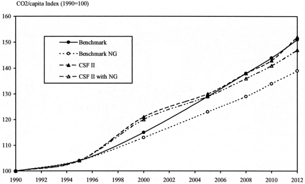
mately 1% higher than its 1990 value Fig. 3 due to rigorous changes in economic infrastructure that lead to a GDP increase of approximately 48% compared to the 1990 levels. As expected, however, this is not the case for the CO₂rcapita index that follows the increase of total CO emissions in a manner similar to that of the2

Ž .

Benchmarkcase Fig. 4 .

Ž .

Finally, it is worth noting that Anton et al. 1996 derived similar results regarding the environmental effects of CSF II in Spain. These authors found that a significant increase in CO emissions should be expected, although they did not₂ take into account changes in energy consumption structure and emission factors. Such changes may have a positive impact stemming from more extensive and effective usage of types of energy that are more friendly to the environment.

5. Concluding remarks

(15)

()

Christodoulakis

et

al.

r

Energy

Economics

22

2000

395

]

422

409

Table 7

a

Ž .

Forecasts of energy demand in Mtoe and percentage deviations from the Benchmarkscenario for theCSF IIandCSF II with NGscenarios

Variable 1995 2000 2005 2008 2010 2012 Average 1990]2012

2008r2012 % changeryear

Ž . Ž . Ž . Ž . Ž . Ž . Ž .

TFC 14.6 0.0 19.2 10.3 22.1 10.0 24.0 10.1 25.6 10.4 27.2 10.7 25.6 10.4 3.2

Ž . Ž . Ž . Ž . Ž . Ž . Ž .

Tradable sector 4.1 0.0 5.5 6.2 6.0 1.5 6.4 1.1 6.7 1.4 7.0 1.7 6.7 1.4 3.4

Ž . Ž . Ž . Ž . Ž . Ž . Ž .

Non-tradable sector 6.1 0.4 8.0 8.5 11.1 19.3 12.9 20.9 14.2 20.9 15.6 20.8 14.2 20.9 3.8

Ž . Ž . Ž . Ž . Ž . Ž . Ž .

Public-agricultural 4.4 0.0 5.5 14.0 5.4 10.6 5.4 10.5 5.4 11.0 5.4 11.7 5.4 11.1 1.4

sectors

Ž . Ž . Ž . Ž . Ž . Ž . Ž .

Oil 11.0 1.9 13.1 6.5 15.2 7.8 16.5 7.5 17.4 7.5 18.5 7.7 17.5 7.6 2.8

Ž . Ž . Ž . Ž . Ž . Ž . Ž .

Electricity 3.0 3.4 3.9 12.3 4.5 10.8 5.0 10.8 5.4 11.0 5.8 11.0 5.4 11.3 4.0

a

(16)

Fig.

1.

Energy

demand

for

Benchmark

and

CSF

II

(17)

()

Christodoulakis

et

al.

r

Energy

Economics

22

2000

395

]

422

411

Table 8

Ž .

Forecasts of CO emissions in Mt , relevant indicators and percentage deviations from the2 Benchmark scenario for the CSF II and CSF II with NG a

scenarios

Variable 1995 2000 2005 2008 2010 2012 Average 1990]2012

2008r2012 %changeryear

CSF II scenario

Ž . Ž . Ž . Ž . Ž . Ž . Ž .

Total CO2 81.6 0.0 96.8 5.8 104.5 1.3 111.7 0.2 116.3 y0.1 123.8 0.2 117.1 0.0 2.2

Ž . Ž . Ž . Ž . Ž . Ž . Ž .

CO2rGDP 0.154 y2.1 0.166 3.6 0.162 y0.8 0.162 y1.9 0.162 y2.2 0.166 y1.9 0.163 y2.1 0.2

Ž . Ž . Ž . Ž . Ž . Ž . Ž .

CO₂rcapita 7.8 0.0 9.2 5.8 9.8 1.3 10.5 0.2 10.8 y0.1 11.5 0.2 10.9 0.0 1.9

CSF II with NG scenario

Ž . Ž . Ž . Ž . Ž . Ž . Ž .

Total CO₂ 81.6 0.0 95.9 4.8 103.5 0.2 109.9 y1.4 114.5 y1.7 120.1 y2.7 114.4 y2.3 2.1

Ž . Ž . Ž . Ž . Ž . Ž . Ž .

CO₂rGDP 0.154 y2.1 0.164 2.6 0.160 y1.8 0.160 y3.5 0.160 y3.7 0.161 y4.7 0.160 y4.3 0.1

Ž . Ž . Ž . Ž . Ž . Ž . Ž .

CO₂rcapita 7.8 0.0 9.1 4.8 9.7 0.2 10.3 y1.4 10.7 y1.7 11.1 y2.7 10.7 y2.3 1.8

a

(18)

()

N.M.

Christodoulakis

et

al.

r

Energy

Economics

22

2000

395

]

422

(19)

()

Christodoulakis

et

al.

r

Energy

Economics

22

2000

395

]

422

413

(20)

()

N.M.

Christodoulakis

et

al.

r

Energy

Economics

22

2000

395

]

422

(21)

CO emissions in Greece, and investigate how those are affected by the implemen-2 tation of the CSF. The forecasts are based on estimated demand equations for

Ž .

each sector of economic activity traded, non-traded, public and agricultural sector

Ž .

and for each type of energy oil, electricity and solid fuels . The energy system is then integrated into a fully-developed macroeconometric model, so that all interac-tions between energy, prices and production factors are properly taken into account.

Our findings suggest that forecast energy demand follows closely forecast output and that the share of electricity in total final consumption rises significantly, while the average annual growth rate of predicted CO₂ emissions for the period 1990]2012 ranges from 1.8% to 2.2%. These rates are higher than world forecasts:

Ž .

Holtz-Eakin and Selden 1995 predict that CO emissions will globally increase by₂ the year 2025 with an average annual rate of 1.8%. As regards the European Union, estimations indicate an annual average increase of 1.1% for the period

Ž

1995]2000, which will come down to 0.5% for the period 2001]2010 Energy in .

Europe, 1996 .

However, it should be stressed that the results, and particularly those obtained for theCSF II andCSF II with NG scenarios, are obtained by assuming a certain amount and type of supply-side effects that stem from the aggregate improvement of various types of infrastructure, private investment and upgrading of human capital. None of those takes specifically into account the effects that individual energy projects financed by CSF II are going to have on the availability, supply and quality of the various types of energy fuels.

More specifically, during the last 4 years a number of activities, which are co-financed by the European Commission and the Greek government, are being implemented within the framework of the Operational Programmes for Energy, Industry and Environmental Protection. Some of these actions will play an impor-tant role in the efforts to restrict the overall growth of emissions of greenhouse gases in Greece.17 _{These actions can be distinguished to those directly related to} improvements of the energy system and to those that primarily target towards

Ž .

environmental protection in Greece including: i energy efficiency improvements Ž .

in the electricity sector and promotion of RES; ii interventions in the industrial sector through the use of more energy efficient production procedures, application Ž . of best available techniques and technologies and increased use of RES; and iii interventions in the transportation sector through the shift towards less polluting forms of transport, improvement of the energy efficiency of vehicles, improvements in road networks and the continuous renewal of the road vehicle fleet, and protection and enhancement of forests.

Ž .

Furthermore, the implementation of the third phase of the CSF CSF III is expected to begin in 2000. Some of its priorities, related to the energy sector, will

17

See Climate Change: The Greek Action Plan for the Abatement of CO and Other Greenhouse Gas2

Ž . Ž .

(22)

be the extension of the NG pipeline network, the interconnection with electricity networks of neighbouring countries, further promotion of RES and co-generation, voluntary agreements with the industrial sector for the promotion of energy efficiency, promotion of the rational use of energy and other infrastructure improvements. Such interventions would enhance the flexibility and the competi-tiveness of the Greek energy system, thus assisting in effectively meeting require-ments arising from the liberalisation of the energy market in Europe. Although, not all of these activities are explicitly targeted towards the reduction of green-house gases, they are expected to drive CO emissions to a much lower level by the₂ period 2008]2012.

Nevertheless, our findings indicate that by the end of the next decade Greece may still be far from the q25% target compared to 1990 levels. An alternative policy tool for the reduction of emissions could be an energy tax imposed on energy consumption. This type of tax } imposed on all energy products in proportionality to their consumption } has two effects: first, it reduces energy consumption through the rise in prices and, second, it increases the general energy price index, thus generating inflationary pressures which result in a loss of competitiveness and a fall in economic activity; the latter effects induces a further fall in energy consumption through output elasticities.18_{An energy tax also affects}

} directly or indirectly } disposable income of households through income taxation. Therefore, the assumption of budget neutrality can be adopted by decreasing the rate of taxation so as to keep the effects on the primary surplus Ždeficit at the benchmark level. Thus, under the assumption of budget neutrality. an energy tax may even have a positive impact on output, if it alleviates other forms of distortionary taxation.

Finally, the provision of the Kyoto Protocol concerning the consideration of a basket of six gases constitutes an element of ‘flexibility’ for the identification of the most cost-effective and environmentally sound policies. Predicted growth rates of CO emissions, illustrated in the present study, indicate that apart from any efforts₂ related to energy sector activities there is also a need in identifying measures that

Ž

would reduce significantly emissions of other gases particularly fluorinated com-.

pounds with high global warming potential . There is, therefore, much scope for the prompt start in the identification and implementation of such initiatives to ensure compliance with the commitments assumed by the end of the period 2008]2012.

Acknowledgements

We have benefited from helpful research assistance by E. Apostolidou and from

18

An alternative solution involves a carbon tax, i.e. an energy tax directly proportional to the carbon

Ž .

(23)

comments on a shorter version of the paper by seminar participants at a confer-ence held at the Athens University of Economics and Business, 10]11 April 1997. The responsibility for any remaining errors is strictly ours.

Appendix A: A model for energy demand in Greece

The model equations are estimated in the two-stage error-correction form ŽEngle and Granger, 1987 : first, the long-run equation estimates are reported. Ž_{followed by the adjusted} _R2 _{and the augmented Dickey} _.

]Fuller unit root test and then the residual Z from the long-run equation is used as an explanatory variable in the short-run equation. Standard errors for the individual parameters are in parentheses. The statistical misspecifation tests following each equation are the following: DW-statistic is the Durbin]Watson test for autocorrelation of order one, the Durbin’s his the autocorrelation test with lagged dependent variable, the Breusch]Godfrey test is for ARrMA processes in the residuals of order 1, the

Ž .

White test is for heteroscedasticity, the augmented 1 lag Dickey]Fuller is for a unit root test in the cointegrating residuals, the Engle ARCH test is for autoregres-sive conditional heteroscedasticity, the Chow test is for parameter stability and the Jarque]Bera test is for normality. Probability values are in brackets. More details

Ž .

on these misspecification tests can be found in Spanos 1986 and Banerjee et al. Ž1993 ..

A.1. Econometric estimates

A.1.1. Sectoral demand

A.1.1.1. Energy demand in the tradable sector Long-run equation

Ž .

logETRs4.86848q 0.76222)logYTRy1

Ž0.74447. Ž0.16919.

w Ž . Ž .x

y 0.19418)log PETRy1rPTRy1 Ž0.06725.

Adjusted R2_s_0.494

w x

Augmented Dickey]Fullers y2.608 0.280

Short-run equation

Ž .

Dlog ETRs 0.00152q 0.79683)Dlog YTRy1 Ž0.01015. Ž0.29980.

w Ž . Ž .x Ž .

y 0.25347)Dlog PETR y1rPTRy1 y 0.44104)Zy1

Ž0.09799. Ž0.23871.

Adjusted R2s0.383

Ž . w x

BreuschrGodfrey LM ARrMA1 s0.468 0.494

w x

(24)

w x Chow tests1.121 0.395

w x

White het. tests5.801 0.760

w x

Jarque]Bera normality tests1.274 0.529

A.1.1.2. Energy demand in the non-tradable sector Long-run equation

w x

ARCH tests0.356 0.551

w x

Chow tests1.521 0.263

w x

A.1.1.3. Aggregate energy demand in the public and agricultural sectors Long-run equation

w x

A.1.2. Demand by type of energy

A.1.2.1. Demand for oil Long-run equation

Ž .

logOILs 3.10565q0.99744)logY y1

(25)

w Ž . Ž .x y 0.21999)log POILy1rPGDPy1

Ž0.06289.

Adjusted R2_s_0.927

w x

Chow test s1.249 0.347

w x

A.1.2.2. Demand for electricity Long-run equation

logELEs y 3.05259q1.75802)logY

Ž_0.47150. Ž_0.07779.

Adjusted R2s0.964

w x

(26)

Adjusted R2s0.144 DW-statistics1.712

A.1.3.2. Price of electricity

Dlog PELEs 0.00228q0.95861)Dlog ULC

Ž_0.01968. Ž_0.07784.

Ž . Ž .

q1y0.95827)Dlog XED)POILF

Adjusted R2_s_0.130 DW-statistics1.466

A.1.3.3. Price of energy in the tradable sector

Dlog PETRs 0.44182)Dlog POILq0.39962)Dlog PELE

Ž0.13244. Ž0.14559.

Ž .

q1y0.44182y0.39962)Dlog PSOL

A.1.3.4. Price of energy in the non-tradable sector

Ž . Ž .

Dlog PENTs 0.75901)Dlog POILq 1y0.75901)Dlog PELEy1

Ž0.09113.

A.1.4. Price linkages

A.1.4.1. Wholesale price index

Dlog WPIs y0.00171q 0.55355)Dlog ULCq0.17779)Dlog PM

Ž0.00769. Ž0.11363. Ž0.15187.

Ž .

q1y0.55355y0.17779)Dlog PE

Adjusted R2_s_0.685 DW-statistics1.670

A.1.4.2. Tradable sector output deflator

Dlog PTRs0.00018q 0.57760)log ULCq0.28757)Dlog PM

Ž0.00927. Ž0.13690. Ž0.18298.

Ž .

q1y0.57760y0.28757)Dlog PE

Adjusted R2s0. 480 DW-statistics1.544

A.1.4.3. Non-tradable sector output deflator

Ž .

Dlog PNTs y0.00758q 0.84016)log ULCq 1y0.84016)Dlog PE

Ž0.00830. Ž0.007765.

(27)

A.1.5. Model identities

A.1.5.1. Demand for solid fuel

Ž .

SOLs ETRqENT1qENT2 yOILyELE

A.1.5.2. Total price of energy

Ž . Ž .

PEsOILr OILqELEqSOL)POILqELEr OILqELEqSOL

Ž .

)PELEqSOLrOILqELEqSOL)PSOL

A.2. List of¨ariables

Name Description Source

ETR Energy demand by the tradable sector trf.

ENT1 Energy demand by the non-tradable sector trf.

ENT2 Energy demand by the public-agricultural sectors trf.

ELE Electricity demand trf.

OIL Oil demand trf.

PE Weighted energy price index trf.

PELE Price of electricity, 1970s1 trf.

PETR Price of energy in the tradable sector, 1970s1 trf. PENT Price of energy in the non-tradable sector, 1970s1 trf.

PGDP GDP deflator, 1970s1 trf.

PM Imports deflator, 1970s1 CEC, trf.

PNT Non-tradable sector price deflator, 1970s1 trf.

POIL Price of oil, 1970s1 trf.

Ž .

POILF Average annual price of oil USD per barrel IFS

PSOL Price of solid fuel, 1970s1 trf.

PTR Tradable sector price deflator, 1970s1 trf.

QYA Agricultural Output, 1970 GDR bn EYSE

ULC Nominal Unit Labour Cost. 1970s1 CEC

VAT Average VAT rate trf.

XED DrachmarDollar exchange rate BG

Y Total output, 1970 GDR bn BG

Ž

YNT Output of non-tradable sector electricity, construction, ESYE

.

transport-communication, trade, banking, dwellings , 1970 GDR bn

Ž

YPS Output of public sector public administration, EYSE

.

health and education, other services , 1970 GDR bn

Ž .

YTR Output of tradable sector manufacture, mining , 1970 GDR bn EYSE

Data sources:

Ž .1 National Accounts, various editions by the National Statistical Service ESYE .Ž .

Ž .2 European Economy, various editions by the Commission of the European Communities CEC .Ž . Ž .3 Centre for Economic Planning KEPE .Ž .

Ž .4 International Financial Statistics, IMF IFS .Ž .

Ž .5 Variables indicated by ‘trf’ in the source column are obtained by transforming original data.

References

(28)

Community Support Framework 1994]1999: Energy Consumption and Associated CO Emissions in2

Spain. FEDEA Working Paper, No. 96-06.

Banerjee, A., Dolado, J., Galbraith, J.W., Hendry, D.F., 1993. Co-integration, Error-correction, and the Analysis of Non-Stationary Data. Oxford University Press, New York.

Boone, L., Hall, S., Kemball-Cook, D., 1992. Fossil fuel demand for nine OECD countries. LBS Discussion Paper, No. 21-92.

Christodoulakis, N., Kalyvitis, S., 1997. The demand for energy in Greece: assessing the effects of the

Ž .

Community Support Framework 1994]1999. Energy Econ. 19 4 , 393]416.

Christodoulakis, N., Kalyvitis, S., 1998a. A four-sector macroeconometric model for Greece and the

Ž .

evaluation of the Community Support Framework 1994]1999. Econ. Model. 15 4 575]620.

Ž .

Christodoulakis, N., Kalyvitis, S., 1998b. The second CSF Delors’ II Package for Greece and its impact on the Greek economy: an ex-ante assessment using a four-sector macroeconometric model. Econ. Plan. 31, 57]79.

Donatos, G.S., Mergos, G.J., 1989. Energy demand in Greece: the impact of two energy crises. Energy

Ž .

Econ. 11 2 , 147]152.

Energy in Europe, 1996. European Energy to 2020: A Scenario Approach. DG XVII for Energy, European Commission.

Engle, R., Granger, C., 1987. Co-integration and error correction: representation, estimation and testing. Econometrica 55, 251]276.

Holtz-Eakin, D., Selden, T.M., 1995. Stoking the fires? CO emissions and economic growth. J. Public2

Econ. 57, 85]101.

Climate Change: The Greek Action Plan for the Abatement of CO2 and Other Greenhouse Gas Emissions, 1995. Ministry for the Environment, Physical Planning and Public WorksrNational Technical University of Athens, Athens.

2nd National Communication to the United Nations Framework Convention on Climate Change, 1997. Ministry for the Environment, Physical Planning and Public WorksrNational Observatory of Athens, Athens.

National Inventory of Greenhouse and Other Gases for the years 1990]1995, 1997. Ministry for the Environment, Physical Planning and Public WorksrNational Observatory of Athens, Athens. PNGC, 1997. Progress of the works for the introduction of natural gas in Greece. Public Natural Gas

Ž .

Corporation in Greek .

Proost, S., Van Regemorter, D., 1992. Carbon taxes in the European Community: design of tax policies

Ž .

and their welfare impacts. Eur. Econ. Special edition 1 , 91]124.

Spanos, A., 1986. Statistical Foundations of Econometric Modelling. Cambridge University Press, Cambridge.