An integral linear interpolation approach to the design
of incremental line algorithms
Chengfu Yao, Jon G. Rokne∗
Department of Computer Science, The University of Calgary, Calgary, Alberta, Canada, T2N 1N4
Received 28 June 1997; received in revised form 12 May 1998
Abstract
A unied treatment of incremental line-drawing algorithms understood from the viewpoint of rounded interpolation, covering Bresenham’s algorithm, run-length algorithms, and multistep versions of both. c 1999 Elsevier Science B.V. All rights reserved.
AMS classication:65Y25; 68R99; 68V05
Keywords:Scan conversion of lines; Integral linear interpolation; Incremental algorithms; Run-length algorithms
1. Introduction
The generation of line segment raster images (called lines hereafter) is an important basic graphics primitive. This is evidenced by the fact that graphics hardware tends to be benchmarked by the speed by which it can generate lines. Considerable interest has therefore been shown in designing ecient line scan-conversion algorithms. These algorithms select the pixels nearest to the line based on the geometry of a line relative to a coordinate grid, an abstraction of the raster display where grid points represent the centers of pixels. Most of the algorithms are incremental algorithms [1–4, 8, 10, 13, 16]. Incremental algorithms are distinguished by the fact that they generate the rastered image of a line from one endpoint of a line to the other by selecting one or multiple pixels in each incremental step along a certain axis (x-axis for the lines with slope between 0 and 1). The choice of which pixels to set is made by testing the sign of a function called a discriminator. The discriminator obeys a simple recurrence formula which may be evaluated using only integer arithmetic and binary shifts. The rst such algorithm was due to Bresenham [2]. His algorithm was easy to implement and it eectively set a standard for subsequent line scan conversion algorithms.
∗Corresponding author. E-mail: [email protected].
The number of pixels generated in each incremental step may be either xed or variable. Algo-rithms which generate a xed number of pixels in each incremental step are usually named according to the length of the incremental step along a chosen axis. We thus have single-step line algorithms which are represented by the rst incremental line algorithm due to Bresenham; the double-step line algorithm of Wu and Rokne [16] and the quadruple-step line algorithm of Bao and Rokne [1]. The double-step algorithm [16] is similar to Bresenham’s algorithm but takes advantage of the special double-step pixel patterns and therefore reduces the number of incremental steps by one half. The quadruple-step algorithm [1] generates four pixels in each incremental step at the cost of one to three decision tests, with the average being slightly less than two. More recently, Graham and Iyengar [11] presented a double- and triple-step incremental line algorithm with which has a double-step line generator potentially being able to set a third pixel in some of the loop iterations. Gill [9] suggested
N-step incremental line algorithms based on Bresenham’s line algorithm. In Bresenham’s algorithm, the sign of a discriminator E predicts the pixel to be chosen at any step. For each possible N-step move, the changes to E for each step in the scan conversion process gives a set of equations that must be satised such that the N-step pattern is next in the sequence making up a line. These equations form a test set that predicts the N-step move in advance.
The incremental line algorithms which generate a variable number of pixels in each incremental step are based on the observation that the rastered image of a line with slope between 0 and 1 can be divided into slices of horizontal runs (pixels with the same ordinate) or diagonal runs (pixels forming a 45◦ segment). A run of pixels is generated in each incremental step. Line algorithms of this type are usually referred to as run-length slice algorithms [4, 8]. A two-state discriminator can be used to determine the length of the next run due to the property that the lengths of the runs are conned to two successive integers except for the rst and the last run. This results in a scheme similar to the one used in algorithms generating xed number of pixels in each step.
The run-length properties were rst proven by Reggiori [12]. In [15] Rosenfeld derived them from the chord property of a straight digital arc, the digitization of a straight line segment. In the horizontal run-length slice line algorithm, the incremental direction is along they-axis for calculating the horizontal runs of the line with slope between 0 and 1 since two consecutive horizontal runs have an increment of one in their ordinates. In [4] Bresenham used the property of the so-called complementary line of a line to calculate the diagonal runs of that line whose slope is between 0.5 and 1. The run-length slice algorithms in [4] can be viewed as a single-step algorithm in the sense that the incremental step is one in the direction of y-axis. Fung, Nicholl and Dewdney [8] presented a double-step version of the run-length slice algorithm to further increase the eciency of line generation. A major drawback of the run-length slice algorithm is the division operation required in the initialization part of the algorithm. A method to avoid division was suggested in [8].
Bresenham’s line algorithm and integral linear interpolation. We then illustrate how variations of the original Bresenham’s line algorithm such as double-step and quadruple-step incremental line al-gorithms can be derived by using double-step and quadruple-step integral linear interpolation. This method also applies to the derivation of the incremental run-length slice line algorithms, however, the discussion of its relation to the linear interpolation is less straightforward.
Careful attention is given to the equal-error problem for each of the algorithms because of its importance for code portability.
Algorithms to perform fast integral linear interpolation have been discussed by Field [5], Rokne and Yao [14], and Graham and Iyengar [11], the latter being a generalization of their double- and triple-step line algorithm [10].
The topics in this paper are well known from other investigations, however, the approach is dierent from other relevant work. This results in a treatment that unies a considerable body of literature on incremental line drawing.
The paper is organized as follows. Section 2 gives some notations and conventions used throughout this paper. Section 3 introduces the technique of integral linear interpolation. Sections 4 and 5 derive the single-step and double-step incremental line algorithms by means of integral linear interpolation. Section 6 uses the integral linear interpolation to derive run-length slice line algorithms. A conclusion is given in Section 7.
2. Notations and conventions
The discussion of the line scan-conversion problem is constrained to lines with slopes between 0 and 1 whose endpoint coordinates are integers. More specically, we denote the two endpoints of the line by (xs; ys) and (xe; ye) and we assume that xe¿xs and ye¿ys. Other lines with integer
endpoints can be transformed to meet this condition via sign changes and=or coordinate swaps. The following notations are used throughout this paper:
1. x=xe−xs and y=ye−ys.
2. In the context of linear interpolation k is used to denote the distance between two consecutive interpolation points. For instance, performing linear interpolation over interval [a; b] with n+ 1 equidistant points including a and b, we have k= (b−a)=n. In the context of line generation, however, k=y=x denotes the slope of the line. In this case k can still be considered as the distance of two consecutive interpolation points in a linear interpolation over interval [ys; ye] with
n=x.
3. ⌊x⌋ denotes the largest integer which is not larger than x;⌈x⌉ denotes the smallest integer which is not smaller than x. ⌊·⌋ and ⌈·⌉ are called the oor and ceiling functions.
4. A letter with a dot accent denotes the integer approximation to a linear interpolation point. The integer which is nearest to an linear interpolation point xi is ˙xi=⌊xi+ 0:5⌋ except when xi has a
fractional part of 0:5. In this case ˙xi=⌊xi⌋ or ˙xi=⌊xi+ 0:5⌋ is acceptable with the latter being the
default choice. We also use ˙xi=⌊xi⌋ or ˙xi=⌈xi⌉ as the integer approximation of xi in situations
where the use of these denitions helps to derive incremental run-length slice line algorithms. 5. c=⌊k⌋.
3. Integral linear interpolation
3.1. Least error integral linear interpolation
The problem of linear interpolation is to nd a set of n+ 1 equidistant points on an interval [a; b], where the lower and upper bounds, a and b, are assumed to be integers for the time being. This is not necessary as the problem itself suggests, however, when this problem is related to line generation, a and b are usually integers or real numbers with some special relation which allows integer arithmetic as we will see in Section 6.
Let us denote the original set of interpolation points by
a=a0; a1; : : : ; an=b;
where ai=a+i(b−a)=n=a+ik for i= 0;1; : : : ; n. Then the integral approximation to the ith point
can be obtained by rounding it to the nearest integer, i.e.,
˙
ai=
a+b−a
n i+ 0:5
(1)
for i= 0;1; : : : ; n. Since ˙ai is obtained by rounding ai to the nearest integer, we call this type of
linear interpolation least error integral linear interpolation. Since
˙
ai=⌊ai+ 0:5⌋; i= 0;1; : : : ; n;
we have
ai−0:5¡a˙i6ai+ 0:5;
ai+1−0:5¡a˙i+16ai+1+ 0:5;
i.e.,
a+ik−0:5¡a˙i6a+ik+ 0:5; (2)
a+ (i+ 1)k−0:5¡a˙i+16a+ (i+ 1)k+ 0:5: (3)
Subtracting Eq. (2) from Eq. (3), we get
k−1¡a˙i+1−a˙i¡ k + 1;
or
k−1¡ a˙i¡ k+ 1:
Ifk is nonintegral, thena˙i can either assume the value⌈k−1⌉=⌊k⌋=cor the value⌊k+1⌋=⌊k⌋+
1 =c+ 1. If k is integral, a˙i=k=⌊k⌋=c. Letting i=ai+1−a˙i−(c+ 0:5) we obtain
˙
ai+1=
a˙
i+c; i¡0;
˙
It follows from n ¿0 that Di= 2ni retains the sign of i. Since Di turns out to be a conveniently
calculated quantity, it is chosen to be the discriminator and we have
˙
ai+1=
a˙
i+c; Di ¡ 0;
˙
ai+c+ 1; Di¿0:
(4)
Noting that
i=ai+1−a˙i−(c+ 0:5)
=a+ (i+ 1)·b−a
n −a˙i−(c+ 0:5);
it follows that
Di= 2na+ 2(i+ 1)(b−a)−2na˙i−n(2c+ 1): (5)
Subtracting Di from Di+1 yields
Di+1−Di= 2(b−a)−2n( ˙ai+1−a˙i):
Hence,
Di+1=
D
i+ 2(b−a)−2nc; Di ¡ 0;
Di+ 2(b−a)−2n(c+ 1); Di¿0:
(6)
The initial value for ˙ai is
˙
a0=a: (7)
Evaluating Eq. (5) for i= 0 determines the initial value of the discriminator
D0= 2(b−a)−n(2c+ 1): (8)
An integerized algorithm for least error integral linear interpolation is thus obtained according to the initial values given by Eqs. (7) and (8) and the recurrence formulas of Eqs. (4) and (6).
3.2. Rounding-up and rounding-down integral linear interpolation
If, instead of dening the integral interpolation points using Eq. (1), we round up each interpolation point ai to the smallest integer which is greater than or equal to ai, i.e., we dene
˙
ai=⌈ai⌉=⌈a+ki⌉ (9)
then we obtain the rounding-up integral linear interpolation.
Analogous to the derivation of the recurrence formulas for the least error integral linear interpo-lation, we can generate similar recurrence formulas for the rounding-up integral linear interpolation with only integer arithmetic. It follows from Eq. (9) that
ai6a˙i¡ ai+ 1; (10)
Proceeding as before we obtain the recurrences
The initial value of the interpolation point is
˙
a0=a (14)
and of the discriminator
D0=b−a−nc: (15)
Similarly, letting ˙ai=⌊ai⌋=⌊a+ki⌋, we dene rounding-down integral linear interpolation. The
recurrence formulas for rounding-down integral linear interpolation are almost the same as the for-mulas for the rounding-up integral linear interpolation and we get
˙
The dierence between (12), (13) and (16), (17) is just in the equality case for the update formulas and in the initial value for D0.
4. Bresenham line algorithm and integral linear interpolation
Consider a line from (xs; ys) to (xe; ye) which lies in the raster plane with an overlaid rectangular
coordinate grid mesh. The line is assumed to meet the conditions imposed in Section 2. Starting from x=xs; y=ys, Bresenham’s algorithm generates the rastered image of a line by increasing
the integer abscissa value by one in each iteration, then deciding which of the two neighboring pixels, (x + 1; y) and (x + 1; y+ 1) is closer to the true line and then moving to that position. The algorithm chooses one of the two pixels by testing the sign of a discriminator. The decision made eectively rounds the real ordinate value of the point on the real line with integer abscissa
x+ 1 to the nearest integer. If an equal error instance occurs, Bresenham’s algorithm will round the real ordinate value up, i.e., choose the integer ordinate to be y+ 1. The discriminator is updated according to a simple recurrence formula. The following code constitutes the core of Bresenham’s line algorithm for generating lines with slopes between 0 and 1.
for (i= 0;i6x; + +i) {
Now let us view the line generation problem from a dierent perspective. Denote the ordered sequence of abscissa of pixels on the line from xs to xe; by X and the ordered sequence of ordinate
of pixels from ys to ye by Y. There is a one to one correspondence between the elements of these
two sequences. Since x¿y, x is increased by one each step a pixel is determined. Hence
X={xs; xs+ 1; : : : ; xe}:
The elements in Y are the results of the least error integral linear interpolation performed on the
interval [ys; ye]:
Y={ys= ˙y
0;y˙1; : : : ;y˙n=ye};
where n=x. In the case ofy ¡ n there exist ˙yi and ˙yi+1 for i= 0;1; : : : ; n−1 such that ˙yi= ˙yi+1. Replacing a; b by ys; ye and n by x in the least error integral linear interpolation formulas obtained
in Section 2.1, we get the following recurrence relations:
˙
The initial value of the discriminator becomes
D0= 2y−(2c+ 1)x: (22)
The relation between Eqs. (20)–(22) and Bresenham line algorithm is revealed by examining the value of c which is trivially determined:
and the initial value of the discriminator becomes
D0= 2y−x: (26)
These recurrence relations are identical to those employed in Bresenham’s algorithm. If c= 1, i.e.,
x=y, the line forms a 45◦ angle with respect to the positivex-direction. The recurrence formulas become
˙
yi+1= y˙
i+ 1; Di¡0;
˙
yi+ 2; Di¿0;
(27)
Di+1=
Di; Di¡0;
Di−2x; Di¿0;
(28)
and the initial value of the discriminator becomes
D0=−x: (29)
These formulas dier from those used in Bresenham’s algorithm. But since the initial value of discriminator is negative, and according to Eq. (28) it will never change in the process of iteration, therefore, according to Eq. (27), the value of ˙yi will increase by one in each iteration to form a 45◦ move. We therefore conclude that least error integral linear interpolation over the interval [ys; ye]
results in a line algorithm which is equivalent to Bresenham line algorithm.
5. Double-step line algorithm and least error integral linear interpolation
5.1. Double-step line algorithm
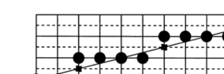
The double-step line algorithm [16] which improves Bresenham’s algorithm is based on the ob-servation that if a point (xi; yi) at the lower left corner of a 2×2 mesh representing an already
plotted pixel in the line with slope between 0 and 1 is given, then only the four pixel patterns shown in Fig. 1 can be formed in a double-step increment in the x-direction under the conditions on the line given in Section 2. Starting from (xs; ys), the x coordinate is now incremented by two raster
units. Then if the pixel at the right-lower (the right-upper) corner of the 2×2 mesh is selected, it is clear that pattern 1 (4) occurs. This means that in each case the middle pixel can be plotted with no extra work. If pattern 2 or 3 occurs (abbreviated pattern 2 (3) in the sequel), then some extra work has to be done in order to distinguish which of the two patterns have to be plotted. It was
conjectured by Freeman [6, 7] and proved by Reggiori [12] (see also [13, 16]) that only two pattern types may occur simultaneously: either 1 and 2 (3) or 2 (3) and 4. This can be proven in a more straightforward manner using the run-length properties of a rastered line which will be discussed in Section 6. From these results the double-step strategy is given by
1. If 06k ¡0:5, then
To distinguish between pattern 2 and 3 requires the test
Di¡
2y; if 06k ¡0:5;
2(y−x) if 0:56k61 (34)
resulting in pattern 2 if the test is passed, pattern 3 if not.
5.2. Designing double-step line algorithm using double-step integral linear interpolation
In this subsection we show that the integral linear interpolation methodology lends itself to the design of double-step line algorithm by extending it to a double-step incremental version. Again the integral linear interpolation used is of the least error type.
Double-step integral linear interpolation was discussed in [14] and we therefore only outline the algorithm for double-step linear interpolation here. We then show its relation to the double-step line algorithm.
same development as in Section 3 we obtain that the formulas to calculate ˙Ai and ˙Di are
and
The above recurrence formulas result directly in a double-step line algorithm since what we really need to calculate is the set of y-coordinates of the pixels on the rastered line, and it is readily understood that this can be achieved by performing double-step linear interpolation over interval [ys; ye]. Replacinga; bby ys; ye, ˙A;a˙by ˙Y ;y˙, and nby x in Eqs. (35) and (36) yields the following
recurrence formulas for calculating y coordinates of the pixels:
˙
Noting that the value of c is determined according to Eq. (23) then the value of C is, from the following equation,
algorithm in [16] for the case of 06k ¡1, and they are correct in the case of k= 1 though the resulting formulas are dierent from those of double-step line algorithm. We omit the derivation here since it is quite easy.
The advantage of using linear interpolation technique in designing double-step line algorithm is obvious. The discussion on double-step pixel patterns and the dierentiation of the two cases depending on the slope of a line being greater or less than 0.5 is no longer needed. Only one set of recurrence formulas is derived which corresponds to dierent sets of formulas derived in [16] depending on the value of C. In an analogous manner we can design a quadruple-step least error integral linear interpolation algorithm, and it is readily understood that quadruple-step line generation [1] is just a special case of quadruple-step least error integral linear interpolation.
6. Run-length line algorithm based on integral linear interpolation
6.1. Horizontal run-length line algorithm
In Sections 2 and 3, we reduced the problem of line generation to the problem of least error integral linear interpolation over the interval [ys; ye] with n=x. An alternative method one would
naturally consider is to reduce the problem of line generation to the problem of performing linear interpolation over the interval [xs; xe] with n=y. Since y6x, this will in general reduce the
number of iteration steps. Unfortunately, this is not helpful as is illustrated by Fig. 2.
The fact that there exist identical elements in the sequence Y when 06k ¡1 is visualized by the horizontal runs of the pixels in the rasterized line. This provides us with a clue for nding the start of each horizontal runs by means of integral linear interpolation since the start of each run has an integral x-coordinate. We impose a set of horizontal mid-lines y=ys+i−0:5; i= 1; : : : ; y (see
Fig. 3). Thex-coordinate of the intersection of the line from (xs; ys) to (xe; ye) with liney=ys+i−0:5
is denoted by xi. It is then readily understood that rasterized image of the half open line segment
whose projection on the x axis is the half open interval [xi; xi+1) is the horizontal run from ⌈xi⌉ to
⌈xi+1⌉ −1. Thus, except for the rst horizontal run which starts from xs, each horizontal run starts
from ⌈xi⌉. To compute ⌈xi⌉ we convert this problem to a problem of rounding-up integral linear
interpolation as introduced in Section 2.2.
Fig. 3. Horizontal run of the pixels in a rasterized line and nding the starting position of each run by rounding-up integral linear interpolation.
Introducing auxiliary point x0=xs−x=2y, we get n+ 1 (n=y) equally spaced points since we
usen mid-lines to intersect the line from (xs; ys) to (xe; ye) (see Fig. 3). The distance betweenxi and
xi+1 is x=y, and the last point is xn=xe−x=2y. Remember that what we really need are the
integer points ˙x1; : : : ;x˙n where ˙xi=⌈xi⌉ is the beginning of (i+ 1)th horizontal run. The beginning of
the rst horizontal run is xs. We now perform rounding-up integral linear interpolation over interval
[x0; xn] to obtain these integer points. Referring to the derivation of the recurrence formulas for
rounding-up integral linear interpolation in Section 2.2, we substitute x0; xn for a andb, respectively.
Here n is changed to y; ai is changed to xi; and c=⌊k⌋=⌊(xn−x0)=n⌋. The lower and upper
bounds of the interval are no longer integers, which seems to be a barrier in performing integral linear interpolation using only integral arithmetic. This diculty can be overcome by examining the equations xn−x0=xe−xs=x. The discriminator Di used is dierent from that dened in Section
2.2. Since
xi+1−x˙i−c=x0+ (i+ 1)
xn−x0
y −x˙i−c
=xs−
x
2y + (i+ 1) x
y−x˙i−c;
we dene
Di= 2y(xi+1−x˙i−c)
= 2yxs−x+ 2(i+ 1)x−2yx˙i−2yc:
Hence,
Di+1−Di= 2x−2y( ˙xi+1−x˙i)
= 2x
−2yc; Di60;
2x−2y(c+ 1); Di¿0:
Let
Fig. 4. A line with equal error cases.
then
yc=x−r; 2y⌊x=2y⌋=x−r˜
and we have the recurrence formulas
˙
xi+1=
˙
xi+c; Di60;
˙
xi+c+ 1; Di¿0;
(44)
Di+1=
D
i+ 2r; Di60;
Di+ 2r−2y; Di¿0:
(45)
The initial values of ˙xi and Di are
˙
x0=
xs−
x
2y
=xs−
x 2y
=xs−(c/1); (46)
D0= 2y(xs−x˙0−c) +x= 2y
x 2y
−2yc+x
=x−r˜−2(x−r) +x= 2r−r;˜ (47)
where / denotes the right binary shift operation.
Equal error instances are treated in a manner consistent with the Bresenham line algorithm as is illustrated in Fig. 4. This is because we use rounding-up to obtain the initial point of the horizontal run. Some properties of a rastered line can be derived directly from Eq. (45):
1. Except for the rst and the last run, the lengths of horizontal runs are conned to two consecutive integers c and c+ 1.
2. The sum of the lengths of the rst and the last horizontal run is either c+ 1 or c+ 2.
3. Pixel patterns 1 and 4 in Fig. 1 cannot occur in one line since the occurrence of pattern 1 implies a horizontal run of length at least 3 and the occurrence of pattern 4 implies a horizontal run of length 1 which is neither the rst nor the last horizontal run of the line. This contradictions property 1.
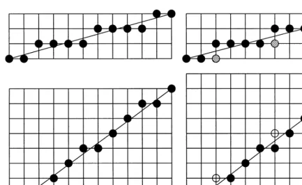
Fig. 5. Lines (bottom) and their complementary lines (top). Diagonal runs in lines are obtained by calculating horizontal runs of the complementary lines. Empty circles in (b) denote the pixels which should be generated by Bresenham line algorithm. This suggest that we use rounding-down integral linear interpolation to calculate the end positions of horizontal runs of the complementary line. The hatched circles denote this adjustment.
6.2. Diagonal run-length algorithm
A rasterized line can be divided into slices of horizontal runs so that multiple pixels can be rendered in each iteration, as shown above. However, when the slope of the line is greater than 0.5, the length of each horizontal run reduces to 1 or 2 since c=⌊x=y⌋= 1. In this case, the advantage of the horizontal run-length algorithm is greatly reduced. In the extreme case of slope being 1, the length of each run reduces to 1 and we actually obtain a single-step algorithm. We can, however, divide the line into diagonal runs since the starting of a new horizontal run is equivalent to a diagonal move of the pixel and each horizontal move of a pixel can be viewed as the starting of a new diagonal run.
The diagonal runs of a line can be obtained by calculating the horizontal runs of its complementary line [4]. For a line with y ¿0:5x, i.e., slope of line ¿0:5, we compute the horizontal runs of its complementary line starting from (xs; ys) and ending at (xe; ye′) where y′e=x−ye, and reverse the
default is a horizontal move (see Fig. 5(b)), resulting in a discrepancy between lines generated by Bresenham line algorithm and lines generated in this manner. This discrepancy can be eliminated by obtaining the horizontal runs through calculating the end positions of the horizontal runs of its complementary line using rounding-down integral linear interpolation and then changing horizontal runs to diagonal runs. Thus ˙xi=⌊xi⌋ is the end of the ith run, and we simply obtain a diagonal run
which ends at abscissa ˙xi. In the case of drawing a line with slope less than or equal to 0.5, we
still use rounding-up integral linear interpolation to calculate the horizontal runs of the line since a rastered line generated in this manner is identical to the rastered line generated by Bresenham’s algorithm no matter if there exist equal error instances.
If we dene
then the derivation of recurrence formulas for the rounding-down integral linear interpolation is similar to the derivation of recurrence formulas for rounding-up integral linear interpolation and we get
Combining the step technique and the run-length technique we can easily derive the double-step run-length line algorithm by using integral linear interpolation. Here we give a brief derivation since the method is almost the same as the method we have used to derive the double-step incremental line algorithm except that we use rounding-up linear interpolation here rather than least error integral interpolation.
Notations used in Section 6.1 will still be used in this section. Dene
Xi=x2i=xs−
Di+1=
D
i+ 2R; Di60;
Di+ 2R−2y; Di¿0;
(53)
where
C=⌊2k⌋=
2x
y
; R= 2xmody;
Di= 2y(Xi+1−X˙i−C)
= 2yxs−x+ 4(i+ 1)x−2yX˙i−2yC:
The initial values of Xi and Di are:
˙
X0= ˙x0=xs−c/1; (54)
D0= 2R−r;˜ (55)
where ˜r=xmod 2y.
To calculate the midpoint ˙x2i+1 between ˙Xi= ˙x2i and ˙Xi+1= ˙x2i+2, we note the fact that ˙x2i+1 = ⌈x2i+1⌉ and the dierence ˙x2i+1−X˙i can be either c or c+ 1. We thus have
˙
x2i+1=
( ˙
Xi+c; x2i+1−X˙i−c60;
˙
Xi+c+ 1; x2i+1−X˙i−c ¿0:
Let
di= 2y(x2i+1−X˙i−c):
Deriving a bit further we get
di=Di−2x+ 2y(C−c):
The formula to calculate ˙x2i+1 is therefore
˙
x2i+1=
( ˙
Xi+c; Di62x−2y(C−c);
˙
Xi+c+ 1; Di¿2x−2y(C−c):
(56)
In the case of ˙Xi+1−X˙i being even, no extra test is need, and we simply have
˙
x2i+1= ˙Xi+m;
where m is an integer and ˙Xi+1−X˙i= 2m.
7. Conclusion
We have presented an approach to the design of incremental line algorithms in this paper which reduces the problem of designing incremental line algorithms to the problem of integral linear in-terpolation over the y extent or the x extent of a line. This new treatment unies a considerable body of literature on incremental line drawing and it has the advantage of simplifying the derivation. The variations of the original Bresenham line algorithm become natural extensions of the algorithm under this framework, and the properties of rastered lines upon which the double-step and the run-length slice line algorithms are based are the direct results of the integral linear interpolation. Further enhancement of existing algorithms, e.g., to incorporate the double-step technique into a run-length slice algorithm, becomes straightforward using this new technique, as is shown in the last subsection.
References
[1] P. Bao, J. Rokne, Quadruple-step line generation, Comput. Graph. 13 (4) (1989) 461– 469. [2] J.E. Bresenham, Algorithm for computer control of digiter plotter, IBM Syst. J. 4 (1965) 25–30. [3] J.E. Bresenham, Incremental line compaction, Comput. J. 25 (1982) 116 –120.
[4] J.E. Bresenham, Run length slice algorithms for incremental lines, in: R.A. Earnshaw (Ed.), Fundamental Algorithms for Computer Graphics, NATO Computer and Systems Series, vol. 17, Springer, New York, 1985, pp. 59–104. [5] D. Field, Incremental linear interpolation, ACM Trans. Graph. (1985) 1–11.
[6] H. Freeman, On the encoding of arbitrary geometric congurations, IRE Trans. EC-102 (1961) 260 –268.
[7] H. Freeman, Boundary encoding and processing, in: B.S. Lipkin, A. Rosenfeld (Eds.), Picture Processing and Psychopictories, Academic Press, New York, 1970, pp. 241–266.
[8] K.Y. Fung, T.M. Nicholl, A.K. Dewdney, A run-length slice line drawing algorithm without division operations, Comput. Graph. Forum 3 (1992) 267–277.
[9] G.W. Gill, N-step and incremental straight-line algorithms, IEEE Comput. Graph. Appl. May (1994) 66 –72. [10] P. Graham, S. Iyengar, Double- and triple-step incremental generation of lines, in: Proc. 1993 ACM Computer
Science Conf., New York, 1993.
[11] P. Graham, S. Iyengar, Double- and triple-step incremental linear interpolation, IEEE Comput. Graph. Appl. May (1994) 49–53.
[12] G.B. Regiori, Digital computer transformations for irregular line drawings, Tech. Rep. 403-22, Department of Electrical Engineering and Computer Science, New York Univ., April 1972.
[13] J. Rokne, B. Wyvill, X. Wu, Fast line scan-conversion, ACM Trans. Graph. 9 (4) (1990) 376 –388. [14] J. Rokne, C. Yao, Double-step incremental linear interpolation, ACM Trans. Graph. 11 (2) (1992) 183–192. [15] A. Rosenfeld, Digital straight line segments, IEEE Trans. Comput. C-23 (1974) 1264 –1269.
![Fig. 2. Linear interpolation over the interval [xs; xe].](https://thumb-ap.123doks.com/thumbv2/123dok/3108507.1377183/11.612.153.358.492.602/fig-linear-interpolation-interval-xs-xe.webp)