Zero distributions for discrete orthogonal polynomials
A.B.J. Kuijlaarsa;∗, E.A. Rakhmanovb;1
aDepartment of Mathematics, City University of Hong Kong, 83 Tat Chee Avenue, Kowloon, Hong Kong b
Department of Mathematics, University of South Florida, Tampa, FL 33620, USA
Received 15 December 1997
Abstract
We give an overview of recent work on the distribution of zeros of discrete orthogonal polynomials. c1998 Elsevier Science B.V. All rights reserved.
AMS classication:33C45; 42C05
Keywords:Zero distribution; Discrete orthogonality; Constrained equilibrium problem
1. Introduction
We begin with the following historical remark. In 1855, Chebyshev [3] considered the problem of polynomial approximation of a function f(x), x∈[−1;1], whose values are obtained by some measurement procedure at N equidistant points
k; N=−1 + 2
k−1
N−1; k= 1; : : : ; N: (1.1)
In other words, values of the function fk; N=f(k; N), k= 1; : : : ; N, are given and we want to nd
a polynomial pn of a smaller degree n¡N representing f in [−1;1]. He used the least-squares
method of approximation, which was known to be very eective. He was looking, therefore, for the polynomial pn(x) with the following minimizing property:
N
X
k=1
k; N(pn(k; N)−fk; N)2= min
degq6n N
X
k=1
k; N(qn(k; N)−fk; N)2;
∗Corresponding author.
1The research of this author is supported by NSF grant DMS 950-1130.
where the numbers k; N¿0 are related to possible errors in the measurement of the values of the
function f.
Most remarkable was the approach to this problem. Chebyshev started with the expansion of the moment series associated with the problem into a continued fraction
Z d(x) z−x =
∞
X
n=0
cn
zn+1 ∼
1|
|z−1
+ 2|
|z−2
+· · ·+ N|
|z−N
; (1.2)
where cn=
R
xnd(x) and
d= dN= N
X
k=1
k; N(k; N): (1.3)
(() is the Dirac delta-function supported at .) Then he proved the fundamental fact that the denominators Qn(x) =xn+· · · of the partial fractions of the continued fraction (1.2) are orthogonal
with respect to :
Z
Qn(x)Qm(x) d(x) = 0; n6=m; n; m¡N: (1.4)
He also proved some basic identities for the polynomials Qn.
The generality of his considerations was clear to Chebyshev and in a series of subsequent papers he obtained similar results for continuous measures
d(x) =w(x) dx: (1.5)
These results may be regarded as the starting point of a ‘general’ theory of orthogonal polynomials. (We note that some special systems were known prior to Chebyshev.) It is interesting to note that the general theory started with the discrete case.
Using this approach, Chebyshev eventually came to the natural representation of the solution of his original problem
pn(x) = n
X
i=0
biQi(x);
where
bi=
1
kQik2
Z
f(x)Qi(x) d(x); kQik=
Z Qi2d
1=2 :
He did not seem to raise the question of the error of approximation kf−pnk, as his whole
work was rather algorithmical. This question leads immediately to the question of the asymptotic behavior of the polynomials Qn(x) =Qn; N(x) as n; N→ ∞. Many approximation problems related
to orthogonal polynomials reduce in the end to a problem of asymptotics.
the literature concerns special discrete orthogonal polynomials, where special properties are used. A heuristic approach to the asymptotics problem for Racah polynomials was used in [21]; in [4] these methods are further developed to make them rigorous. In [27, 28] explicit formulas for Krawtchouk and Hahn polynomials were used to obtain (may be, the rst) rigorous results on strong asymptotics for some cases where n=N→0. More recently, uniform asymptotic expansions of Charlier and Meixner polynomials were given in [13, 25]. In coding theory, there is an interest in the asymptotics of extreme zeros of certain discrete orthogonal polynomials like Krawtchouk polynomials, see e.g. [16] and the references given there. Strong asymptotics for these polynomials was obtained with the help of their generating function in [12]. For general information on discrete orthogonal polynomials we refer the reader to monographs [5, 20, 30].
This paper is devoted to recent progress on the problem based on general potential theoretic considerations. The present development started with Rakhmanov [23] who realized that a new kind of equilibrium problem governs the asymptotics of discrete orthogonal polynomials. This was pursued further by Dragnev and Sa [9] and Kuijlaars and Van Assche [14]. We give a survey of the new ideas that are involved, and about connections with other recent work. We have included a number of conjectures, which we hope, may lead to a growing interest in the asymptotic properties of discrete orthogonal polynomials.
2. Constrained equilibrium measure
A general approach to the problem of zero distribution for polynomials Qn; N dened by (1.3)–
(1.4) was developed in [23]. The idea of the method is based on the following observation. Suppose
n; N→ ∞ in a certain way, e.g.,n→ ∞ andN=Nn→ ∞. Typically, we have that n=Nn→c∈(0;1).
Suppose next that the counting measure for supp(N) is weakly convergent:
ˆ
n; N=
1
n
N
X
k=1
(k; N)
∗
−→: (2.1)
The normalization by 1=n is related to the normalization for the counting measure of the zeros of Qn; N in (2.2). Then, if we select any weakly convergent subsequence of the sequence of zero
counting measures for Qn; N
(Qn; N) :=
1
n X
Qn; N(x) = 0
(x)−→∗ (2.2)
(as n→ ∞; n∈⊂N), we necessarily have d6d, because Qn; N has at most one zero in any
interval [k; N; k+1; N].
This suggests that the limit zero distribution may be described by a well-known equilibrium problem on the support of as in the case of orthogonality with respect to a weight function, but in the ‘restricted’ class of measures
Indeed, this is true under an additional ‘separation’ condition for the points {k; N} as stated in
Theorem 3.1 in the next section. An important part of the proof of this theorem is the following result containing characteristic properties of the constrained equilibrium measure. We use the notations
J() =
Z Z
log 1
|x−y|d(x) d(y);
V(x) =
Z
log 1
|x−y|d(y)
to denote the energy and the potential of , respectively. S= supp() denotes the closed support
of .
Theorem 2.1. Let be a positive measure with continuous potential V and kk¿1; S
==
[−1;1]. Then each of the following conditions uniquely determines the same unit measure =
∈M.
(1) J() = min∈MJ()
(2a) There is a constant w such that
V(x)¿w; x
∈S−;
V(x)6w; x∈S:
(2b) There is a constant w such that
V(x) =w; x ∈S−;
V(x)6w; x∈:
(3) minx∈S−V
(x) = max
∈Mminx∈S −V
(x):
We call the equilibrium measure with constraint . We note that the condition (2a) or (2b)
uniquely denes the pair= and w=w. We have presented a simplied version of the existence
theorem. The condition S= [−1;1] may be replaced by the assumption that S is a compact set of
positive capacity and the condition of continuity of V may be omitted. In this case, the relations
(2a) and (2b) hold quasi-everywhere over the indicated sets and the min in (3) has to be replaced by essmin.
The proof of Theorem 2.1 follows standard potential theoretic arguments. The set M is compact
in the weak topology and the energy functional is strictly convex. This implies the existence and uniqueness of the measure satisfying the condition (1). A standard variational technique for the energy functional J shows that conditions (1) and (2a) are equivalent. Next, (2b) follows from (2a) and the fact that S=. Indeed, suppose there exists a point x0∈\S. We have that
V(x) is subharmonic in C
\S and hence, by the maximum principle for subharmonic functions,
V(x
0)¡maxSV
3. Zero distribution of discrete orthogonal polynomials
We return to the triangular table of polynomials Qn; N(x) =xn+· · · dened by the orthogonality
conditions
Z
Qn; N(x)Qm; N(x) dN(x) = 0; n6=m; n; m¡N; (3.1)
with respect to a sequence of discrete measures
dN= N
X
k=1
k; N(k; N): (3.2)
Theorem 3.1 (Rakhmanov [23]). Suppose that the following conditions are satised as n; N→ ∞.
(i) ˆn; N=
(iii) There exists ¿0 such that
|k+1; N −k; N|¿
In \S− we have =, which means that Qn; N has about as many zeros as supp(n; N). It is
Now, the weak convergence of (Qn; N) to implies the following convergence of polynomials:
|Qn; N(x)|1=n= exp{−V(Qn; N)(x)} → exp{−V(x)}: (3.7)
Would this convergence be uniform, then we could easily derive from (3.6), (3.7) that
lim
Actually, we have only convergence in capacity and semiuniformal from above in (3.7) which gives an upper bound
neighborhood of this point contains much more points of supp(n; N) than zeros ofQn; N. This enables
us to select for any large enoughn, a point n=kn; N∈supp(n; N) such that n→x0 and the distance
from n to the zeros of Qn; N is at least =(2N). Some estimates show that we then have
|Qn; N(n)|1=n→e−V
(x 0):
This gives the lower bound complementing (3.9) and hence proves the equality (3.8).
Finally, the minimal possible number in the right-hand side of (3.8) occurs when = according
to the min-max property of , see condition (3) from Theorem 2.1.
Formally, it is convenient to separate the lower bound and the upper bound in the above scheme. So the formal proof is based on the following two lemmas.
Lemma 3.2. Let pn(x) =xn+· · · be any sequence of polynomials with (pn)
∗
−→. If the
condi-tions of Theorem 3.1 are satised; then
4. Equilibrium with external eld and zero distribution of orthogonal polynomials with varying weights
Considerable progress in the theory of continuous orthogonal polynomials in the period 1980– 1995 was achieved by the application of equilibrium distributions with external eld, see [11, 17– 19, 22, 26]. We present here two basic theorems in this direction which should be compared with Theorems 3.1 and 2.1 above. For simplicity we restrict ourselves to the case where is a closed interval, which may be bounded or unbounded.
Let (x) be a continuous function on satisfying the condition
lim
|x|→∞
(x)
log|x|= +∞ (4.1)
in case is unbounded, and letM denote the class of all positive unit measures on with compact
support.
Theorem 4.1. Each of the following conditions uniquely denes the same unit measure=∈M.
(1) J() + 2
Z
d= min
∈M
J() + 2
Z d
:
(2) There is a constant w such that
V(x) +(x) =w; x ∈S;
V(x) +(x)¿w; x∈:
(3) min
(V
+) = max ∈Mmin (V
+):
The measure is usually called the (unit) equilibrium measure with external eld . We note that
condition (2) uniquely denes the pair = and w=w.
Now, suppose the polynomials Qn(x) =xn+· · · are dened by the orthogonality relations
Z
Qn(x)xjn(x) dx= 0; j= 0;1; : : : ; n−1
with respect to weight functions n(x)¿0 depending on the degree of the polynomials.
Theorem 4.2. If the sequence n(x)1=n is uniformly convergent
n(x)1=n→(x) = e−2(x); x∈;
and satises (4.1), then
(Qn)
∗
−→:
Comparison of conditions (1)–(3) of Theorem 4.1 dening the equilibrium measure with external eld with conditions (1)–(3) of Theorem 2.1 dening the constrained equilibrium problem suggests a close relation between the two concepts. Indeed, we will show in the next section that constrained problems may be reduced to an equilibrium with external eld.
5. Reduction of the constrained equilibrium problem to an equilibrium problem with external eld
The second assertion of Theorem 4.1 may be formulated in a slightly more general form taking into account the possibility of an arbitrary normalization of the equilibrium measure . Namely,
given an external eld and a positive number t¿0, there exists a unique positive measure=t;
satisfying
Vt; (x) +(x) =w
t; ; x∈S;
Vt; (x) +(x)¿w
t; ; x∈;
(5.1)
and kk=t.
On the other hand, the second statement of Theorem 2.1 says that the unit -constrained equilib-rium measure is uniquely dened by
V(x) =w; x∈S;
V(x)6w; x∈=S;
(5.2)
which can also be written in the form
V−
(x)−V(x) =
−w; x ∈S;
V−(x)−V(x)¿−w; x∈: (5.3)
Hence with (x) =−V(x), x∈,
t; = −, t=kk −1, the relations (5.1) and (5.3) are
equivalent. We have obtained the following result.
Theorem 5.1 (see also [9, 23]). With t=kk −1; (x) =−V(x); x∈; we have
=−t;; w=−wt; :
Explicit formulas for the support of t; and the density of this measure are known, at least in
the case when suppt; is an interval. This holds, for example, if is a convex function, but this
condition is not necessary (see [1, 17, 26]).
Theorem 5.2. If is a convex function; then St; = [t; t] where t; t are roots of the system of
equations
1
Z t
t
′(x) dx
p
(t−x)(x−t)
= 0; 1
Z t
t
x′(x) dx
p
(t−x)(x−t)
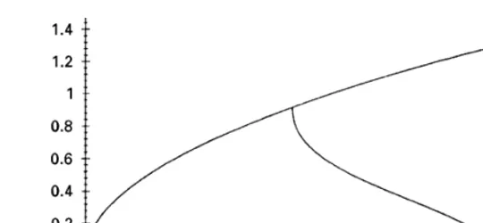
Fig. 1. Zero distributions of discrete Chebyshev polynomials.
For the density of t; ; we then have
dt;
dx = q
(t−x)(x−t)
1
2 Z t
t
′(y)−′(x)
y−x
dy p
(t−y)(y−t)
:
These results enable us to obtain an explicit representation for a rather wide class of measures
. We restrict ourselves to one example from [23].
Theorem 5.3. If d(x) = dx=(2c); x∈[−1;1] where c∈[0;1] and r=√1−c2; then
d
dx =
1
2c; x∈[−1;−r]∪[r;1];
1
carctan
c
√
r2−x2; x∈[−r; r]:
This measure represents the zero distribution as n; N→ ∞; n=N→c of discrete Chebyshev
poly-nomials given by (3.1)–(3.2) with k; N dened by (1.1) and k; N= 1.
See Fig. 1 for the density of the zero distributions of discrete Chebyshev polynomials correspond-ing to c= 0, 0:4, 0:6 and 0:8. Observe that the constraint is active on the intervals [−1;−r] and [r;1].
6. Discrete orthogonal polynomials with exponentially varying weights and constrained equilibrium with external eld
equilibrium problem with external eld was also studied in [7] in connection with the continuum limit of the nite, non-periodic Toda lattice.
Theorem 6.1 (Dragnev and Sa [9]). Let be a positive measure whose support S= is an
interval. Suppose kk¿1 and for every compact K⊂; the restriction of toK has a continuous
potential. Let be a continuous function on such that (x)−log|x| tends to +∞ as |x| → ∞;
in case is unbounded. Then each of the following conditions uniquely denes the same unit
measure =
and the constant w are used in the following generalization of Theorem 3.1.
Theorem 6.21 (Dragnev and Sa [9]). Suppose the polynomials Q
n; N are dened by (3.1)–(3.2),
where the measures N are supported on the bounded interval = [a; b]. Let n; N→ ∞ in such a
way that the following hold:
(i) ˆn; N=
(iii) There exists a constant ¿0 such that
|k+1; N −k; N|¿
After nishing this paper; we learned that Theorem 6.2, which we quoted from an early manuscript of [9] available to us;was revised in the nal version of [9]. The separation condition (iii) has been replaced by the considerably weaker condition
(iii′) (1=n) log|R′
N(k; N)| → −V(x) if k; N→x; k=kN;
where RN(x) =Qk(x−k; N) is the interpolating polynomial of the points k; N. See Section 8 below, for another
(con-jectured) separation condition that might replace (iii). It is an interesting problem to determine the relation between (iii′)
and
The proofs of Theorems 6.1 and 6.2 in [9] essentially follow the proofs of Theorems 2.1 and 3.1 in [23]. In the case that in Theorem 6.1 is unbounded, an additional argument is needed to show that the measure
is supported on a compact set.
Finding explicit solutions of combined equilibrium problems is getting more complicated because it is possible now that S
See [9] for more detailed results.
In [9, 10] the equilibrium measures
were computed with contracted Krawtchouk polynomials Qn; N which are orthogonal with respect to the measure
dN=
Following [9], we present here the explicit formulas for this measure for p=q=1
2. See [10] for
2, the constraint is not active, while for c¿ 1
2, the constraint is active on [0; r]∪[1−r;1].
In all cases, the free part of
7. Discrete orthogonality on countable sets
A further generalization was provided in [14] to the case of orthogonal polynomials on countable sets. The polynomials Qn; N(x) =xn+· · · are assumed to be orthogonal with respect to the measure
dN=
∞
X
k=1
k; N(k; N):
HereN does not refer to the number of points in the support of N as before, but is just a parameter.
The following result is an extension of Theorems 3.1 and 6.2 to orthogonality on countable sets. While it is not stated as such in [14] it is easily derived from the results obtained there.
Theorem 7.1. Let be an unbounded interval. Let n; N→ ∞ in such a way that the following hold:
(i) ˆn; N=
1
n
∞
X
k=1
(k; N)
∗
−→;
where satises the conditions of Theorem 6.1. The weak∗ convergence is with respect to
con-tinuous functions on with compact support.
(ii) 1k; N=n −e−2(k; N)→0
uniformly for k in{k:k; N∈K} for every compact subset K of . Here is a continuous function
on such that (x)−log|x| →+∞ as |x| → ∞.
(iii) There exists a continuous function on ; which is positive on \E where E has capacity
zero; such that
|k+1; N −k; N|¿
(k; N)
N ; k= 1;2; : : : :
(iv) There exist two positive functions A(x) and B(N) such that
#{k: k; N∈[−x; x]}6A(x)B(N);
where A and B satisfy
lim
|x| → ∞
logA(x)
|x| = 0;
for every ¿0; and
lim
N→ ∞
logB(N)
N = 0: Then
(Qn; N) =
1
n X
Qn; N(x) = 0
and
where the measure
and the constant w are as in Theorem 6.1.
Note that the separation condition (iii) has been relaxed. It allows the separation constant to vary withx and, more importantly, to vanish at a small set (capacity zero), for example at a discrete set of points. The condition (iv) is needed to control the contribution to the L2 norm of Q
n; N from
points that are far away (close to innity).
If is unbounded, the constrained equilibrium problem with external eld is in general dicult to solve explicitly. Since S
is a compact set, it can never be equal to , and therefore the reduction
formula (6.1) does not hold. However, in some cases, one can make an educated guess to nd the explicit solution. This was done in [14] where explicit formulas were obtained for ‘discrete Freud weights’
are orthogonal with respect to the measures
dN=
In [14] it was shown that there exist constants B¿A¿0, depending on ; ; such that
Fig. 2. Density of zeros and constraint for discrete Freud weights with= 3=2.
See Fig. 2 for the density of the zero distribution for discrete Freud weights corresponding to =3 2,
A= 1 and B= 2, together with the density of the constraint . Observe that the constraint is active on the interval [0; A].
The density (7.2) is known as a Nevai–Ullman density and was found before in [31, pp. 123–124] as the density of the contracted zero distribution of polynomials Pn generated by the recurrence
Pn+1(x) = (x−bn)Pn(x)−a2nPn−1(x); n¿1;
with P0(x) = 1, P1(x) =x, and recurrence coecients satisfying
an
n1=→
B−A
4 ;
bn
n1=→
A+B
2 :
As the orthogonal polynomials Qn associated with (7.1) have the same contracted zero distribution,
it is natural to pose the following problem, which may be called the ‘discrete Freud conjecture’:
Conjecture 1. The orthogonal polynomials Qn(x) =xn+· · · associated with the discrete measure
(7.1) satisfy the recurrence
Qn+1(x) = (x−bn)Qn(x)−a2nQn−1(x); n¿1;
with
an
n1=→
B−A
4 ;
bn
n1=→
A+B
2 :
8. Remarks on the separation condition
The separation condition (iii) is a common element in all the convergence Theorems 3.1, 6.2 and 7.1 above. In this section we discuss briey the status of this condition.
Conjecture 2. The condition (iii) in Theorems 3.1 and 6.2 may be replaced by the following
condition:
J∗( ˆn; N) =
1
n2
X
j6=k
log 1
|k; N −j; N|→
J(): (8.1)
(J∗() is the discrete energy of the discrete measure.) It is easy to show that (iii), together with
(i), implies (8.1). Therefore, (8.1) is a more general condition than (iii). We consider an example in order to show that (8.1) is essentially weaker than (iii).
We select a sequence of numbers N∈(0;1=N) and dene 2N points k;2N, k= 1; : : : ;2N by
2k−1;2N= −1 + 2
k−1
N−1−N; 2k;2N= −1 + 2
k−1
N−1+N; for k= 1; : : : ; N. Let
N=
1 2N
2N
X
k=1
(k;2N)
and let Qn; N(x) =xn+· · · be the associated orthogonal polynomials. Supposen; N→ ∞ with n=(2N) →c∈[0;1]. Then we have
ˆ
n; N=
1
n
2N
X
k=1
(k;2N)
∗
−→ d=1
cdx:
The conditions (i) and (ii) of Theorem 3.1 are satised, but it is possible to prove that if
lim
N→ ∞ 1=N
N =¡1
the assertion of the theorem is not true. Actually, it may be shown that, for small enough,
(Qn; N)
∗
−→=2:
This shows that the separation condition (iii) cannot be omitted completely in Theorem 3.1. We can only look for weaker conditions.
Next, if limN→ ∞1N=N = 1, the condition (8.1) is satised. Therefore, if the conjecture is correct,
the assertion of Theorem 3.1 remains valid. However, the separation condition (iii) is violated already (also in the more general form of Theorem 7.1) if limN→ ∞NN= 0. This shows that (8.1)
is essentially weaker than condition (iii).
Finally, we note that (8.1) cannot be used in cases where supp(n) is a countable set, since
J∗( ˆn; N) may be innite. The Conjecture 2 has to be modied as follows.
Conjecture 3. The condition (iii) in Theorem 7.1 may be replaced by
J∗( ˆn; N|E)→J(|E); (8.2)
where E is some open set containing the support of
9. Varying recurrence coecients
Very recently, an alternative approach to nding zero distributions of orthogonal polynomials was given in [15]. This approach is based on the coecients in the three-term recurrence, and as such its usefulness is limited to those orthogonal polynomials for which the recurrence is known explicitly.
Theorem 9.1 (Kuijlaars and Van Assche [15]). Let for each N; Qn; N(x) =xn+· · · be a sequence
of polynomials satisfying the three-term recurrence
Qn+1; N(x) = (x−bn; N)Qn; N(x)−a2n; NQn−1; N(x) (9.1)
with an; N¿0 and bn; N∈R. Suppose there exist continuous functions a(t) and b(t) such that
an; N→a(t); bn; N→b(t)
whenever n; N→ ∞ in such a way that n=N→t¿0.
Then; as n; N → ∞ with n=N→c¿0;
(Qn; N)
∗
−→ 1c
Z c
0
![(t); (t)]dt; (9.2)
where
(t) =b(t)−2a(t); (t) =b(t) + 2a(t) (9.3)
and ![; ] is the measure on [; ] with density
d![; ]
dx =
1
p(−x)(x−)
; ¡x¡:
This result was obtained earlier in [7] under more restricted conditions on (t) and (t).
The measure in the right-hand side of (9.2) is an average of the (unweighted) equilibrium mea-sures for varying intervals. It is interesting to note that a similar representation was found in [23] for the solution of certain equilibrium problems with external elds, see also [1, 2].
For classical orthogonal polynomials of a discrete variable, the recurrence coecients are known explicitly and Theorem 8.1 can be used to obtain the zero distributions. In many cases the integral in (9.2) can be evaluated and we obtain an explicit expression.
For example, for discrete Chebyshev polynomials (3.1)–(3.2) with k; N= 1 and k; N given by
(1.1), the recurrence coecients are
an; N=
n√N2−n2
(N −1)√(2n−1)(2n+ 1); bn; N= 0:
In this case the recurrence terminates at n=N, but Theorem 8.1 remains valid provided that c61. Letting n=N→t we nd a(t) =√1−t2=2 and b(t) = 0, so that
Thus if n=N→c61,
The integral is easy to evaluate and we get the result of Theorem 5.3.
In a similar way, one can nd the zero distributions associated with Krawtchouk polynomials and many other special systems of orthogonal polynomials, see [15].
We now describe how the measure in the right-hand side of (9.2) may appear as the solution of a constrained equilibrium problem with external eld. We assume that a(t) andb(t) are continuous functions and (t) and (t) are given by (9.3). Following [7], we assume that the functions (t) and (t) satisfy the following conditions.
(i) (t) has at most one extremum, which, if it exists, is a minimum. (ii) (t) has at most one extremum, which, if it exists, is a maximum.
In all examples arising from known systems of orthogonal polynomials these conditions were found to be satised [15].
For each x, we put
t−(x) = inf{t¿0: x∈[(t); (t)]};
which could be innite. We also dene
0(x) =
the constrained equilibrium problem with external eld and constraint has the solution
We note that for the potential of the measure ![; ], we have
third line of (9.6) by (9.9) and the non-negativity of the Green function. By Theorem 6.1 (2) the relations (9.6) imply that =
and the theorem is proved.
We note that the external eld (9.4), being an integral of Green functions, is similar to the external elds considered in [1], see also the survey [18]. This relation is not yet completely understood.
It is clear that the support of the constrained equilibrium measure =c=c is given by
S=
It is also clear from the proof of Theorem 8.2 that the constraint =T=c is not active if the
function (t) is decreasing on [0; c] and (t) is increasing on [0; c]. If (t) is not decreasing on the interval [0; c], then it must take its minimum value min at a point in [0; c]. Then the constraint is
active on the interval [min; (c)]. Similarly, if assumes its maximum value max in [0; c], then the
constraint is active on [(c); max]. In all cases the ‘free’ part of is supported on [(c); (c)].
10. Bounds for polynomials with a unit discrete norm
In this last section, we report on recent progess on the problem how to estimate the norm of a polynomial from bounds on its values on a nite set. We restrict our remarks to the case of the uniform norm and equidistant points. Let
k; N= −1 + 2
k−1
and let pn(x) be a polynomial of degree n with
|pn(k; N)|61; k= 1; : : : ; N: (10.2)
What can we say about bounds for |pn(z)| at a point z∈C?. The question is closely related to
the discussion above and is, in particular, important in the connection with the study of strong asymptotics for discrete orthogonal polynomials. In addition, many approximation problems (in particular, the one mentioned in Section 1 of this paper) also depend on this problem.
It was proven in [6] that, if n6C√N, then |pn(x)|6C1, x∈[−1;1] and this result is sharp in
the sense that if n=√N→ ∞, then max[−1;1]|pn(x)| may grow like exp(Cn2=N), (see [6] for details
and further references).
The above discussion of discrete orthogonal polynomials suggests that conditions (10.1)–(10.2) imply much better bounds for |pn(x)| on the support of the free part of the constrained equilibrium
measure , ( d=N=(2n) dx), than on the whole interval [−1;1]. Indeed, we have
Theorem 10.1 (Rakhmanov [24]). Under conditions (10.1)–(10.2) we have
|pn(z)|6Clognexp{w−V
(z)}; z∈C; (10.3)
where d=N=(2n) dx. In particular;
|pn(x)|6Clogn; |x|6
q
1−(n=N)2; x∈R: (10.4)
Moreover, the extra factor logn may be eective only near the extreme points ±p
1−(n=N)2 of
supp(−). For instance, we have
Theorem 10.2 (Rakhmanov [24]). Under conditions (10.1)–(10.2) we have
|pn(x)|6Clog
1
1−x2−(n=N)2; |x|6
q
1−(n=N)2: (10.5)
More general results of this kind are contained in [24]. However, rather restrictive conditions on the points {k; N} are required to get estimates like (10.3)–(10.5). In [8] bounds for |pn(z)|1=n are
obtained under much more general conditions (like those in Theorem 6.2).
Acknowledgements
We thank S.B. Damelin, P.D. Dragnev, M.E.H. Ismail, K.T-R. McLaughlin, E.B. Sa, W. Van Assche and R. Wong for useful discussions.
References
[1] V.S. Buyarov, Logarithmic asymptotics of polynomials that are orthogonal on R with nonsymmetric weight, Mat.
Zametki 50 (1991) 28–36, English transl. in Math. Notes 50 (1991) 789–795.
[3] P.L. Chebyshev, Interpolation of equidistant nodes, and, on continued fractions, in: Complete Works, USSR Academy of Sciences Publishing House, Moscow–Leningrad, 1948; French transl., Oeuvres, Chelsea, New York, 1962. [4] L-C. Chen, M.E.H. Ismail, Asymptotics of Racah coecients and polynomials, manuscript.
[5] T.S. Chihara, An Introduction to Orthogonal Polynomials, Gordon and Breach, New York, 1978.
[6] D. Coppersmith, T.J. Rivlin, The growth of polynomials bounded at equally spaced points, SIAM J. Math. Anal. 23 (1992) 970 –983.
[7] P. Deift, K.T-R. McLaughlin, A continuum limit of the Toda lattice, Mem. Amer. Math. Soc. 131 (1998). [8] S.B. Damelin, E.B. Sa, Asymptotics of weighted polynomials on varying sets, manuscript.
[9] P.D. Dragnev, E.B. Sa, Constrained energy problems with applications to orthogonal polynomials of a discrete variable, J. Anal. Math. 72 (1997) 223–259.
[10] P.D. Dragnev, E.B. Sa, A problem in potential theory and zero asymptotics of Krawtchouk polynomials, manuscript. [11] A.A. Gonchar, E.A. Rakhmanov, Equilibrium measure and distribution of the zeros of extremal polynomials, Mat.
Sb. 125 (1984) 117–127; English transl. in Math. USSR-Sb. 53 (1986) 119 –130. [12] M.E.H. Ismail, P. Simeonov, Strong asymptotics for Krawchuk polynomials, manuscript. [13] X.S. Jin, R. Wong, Uniform asymptotic expansions for Meixner polynomials, manuscript. [14] A.B.J. Kuijlaars, W. Van Assche, Extremal polynomials on discrete sets, manuscript.
[15] A.B.J. Kuijlaars, W. Van Assche, The asymptotic zero distribution of orthogonal polynomials with varying recurrence coecients, manuscript.
[16] V.I. Levenshtein, Krawtchouk polynomials and universal bounds for codes and design in Hamming spaces, IEEE Trans. Inform. Theory 41 (1995) 1303–1321.
[17] G. Lopez, E.A. Rakhmanov, Rational approximations, orthogonal polynomials and equilibrium distributions, in: Alfaro et al. (Eds.), Orthogonal Polynomials and their Applications Lecture Notes in Math., vol. 1329, Springer, Berlin, 1988, pp. 125 –156.
[18] D.S. Lubinsky, An update on orthogonal polynomials and weighted approximation on the real line, Acta Appl. Math. 33 (1993) 121–164.
[19] H.N. Mhaskar, E.B. Sa, Extremal problems for polynomials with exponential weights, Trans. Amer. Math. Soc. 285 (1984) 203–234.
[20] A.F. Nikiforov, S.K. Suslov, V.B. Uvarov, Classical Orthogonal Polynomials of a Discrete Variable, Springer, Berlin, 1991.
[21] G. Ponzano, T. Regge, Semiclassical limit of Racah coecients, in: Spectroscopic and Group Theoretical Methods in Physics, North-Holland, Amsterdam, 1969, pp. 1–58.
[22] E.A. Rakhmanov, On asymptotic properties of polynomials orthogonal on the real axis, Mat. Sb. 119 (1982) 163–203; English transl. in Math. USSR-Sb. 47 (1984) 155–193.
[23] E.A. Rakhmanov, Equilibrium measure and the distribution of zeros of the extremal polynomials of a discrete variable, Mat. Sb. 187 (1996) 109 –124; English transl. in Sb. Math. 187 (1996) 1213–1228.
[24] E.A. Rakhmanov, On bounds for polynomials with unit discrete norms, manuscript.
[25] B. Rui, R. Wong, Uniform asymptotic expansion of Charlier polynomials, Meth. Appl. Anal. 1 (1994) 294 –313. [26] E.B. Sa, V. Totik, Logarithmic Potentials with External Fields, Springer, New York, 1997.
[27] I.I. Sharapudinov, Asymptotic properties of Krawtchouk polynomials, Mat. Zametki 44 (1988) 682– 693; English transl. in Math. Notes 44 (1988) 855– 862.
[28] I.I. Sharapudinov, Asymptotic properties of the Hahn orthogonal polynomials of a discrete variable, Mat. Sb. 180 (1989) 1259 –1277; English transl. in Math. USSR-Sb. 68 (1991).
[29] H. Stahl, V. Totik, General Orthogonal Polynomials, Cambridge University Press, Cambridge, 1992.
[30] G. Szeg˝o, Orthogonal Polynomials, AMS Colloquium Publications 23, 4th ed., Amer. Math. Soc., Providence, RI, 1975.