Global Patch Matching
Xu Huang a, b, * , Kun Hu c, *, Xiao Ling d, Yanfeng Zhang d, Zhengwu Lu a, Gang Zhou a a Wuhan Engineering Science & Technology Institute, Jiangda Road 30, Wuhan, China b Wuhan Sense Tour Tecnhonogy Company, Luoshi South Road 320, Wuhan, China
c Key Laboratory of Technology in Geo-spatial Information Processing and Application System, Institute of Electronics, Chinese Academy of Sciences, Beijing 100190, China
d School of Remote Sensing and Information Engineering, Wuhan University, China
Commission II, WG II/I
KEY WORDS: Patch Matching; Matrix Energy Function; Global Optimization; Fronto-parallel Bias; 3D Label Algorithm
ABSTRACT:
This paper introduces a novel global patch matching method that focuses on how to remove fronto-parallel bias and obtain continuous smooth surfaces with assuming that the scenes covered by stereos are piecewise continuous. Firstly, simple linear iterative cluster method (SLIC) is used to segment the base image into a series of patches. Then, a global energy function, which consists of a data term and a smoothness term, is built on the patches. The data term is the second-order Taylor expansion of correlation coefficients, and the smoothness term is built by combing connectivity constraints and the coplanarity constraints are combined to construct the smoothness term. Finally, the global energy function can be built by combining the data term and the smoothness term. We rewrite the global energy function in a quadratic matrix function, and use least square methods to obtain the optimal solution. Experiments on Adirondack stereo and Motorcycle stereo of Middlebury benchmark show that the proposed method can remove fronto-parallel bias effectively, and produce continuous smooth surfaces.
1. INTRODUCTION
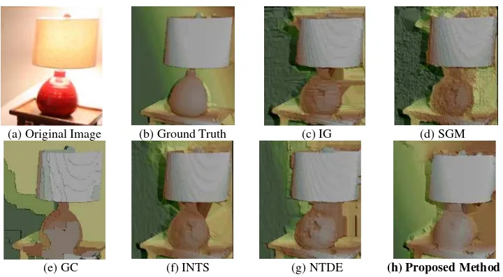
Stereo dense matching has been attracting increased attentions in the photogrammetry and computer vision communities for decades (Scharstein and Szeliski, 2002). Most stereo dense matching algorithms assume fronto-parallel planes and assign one label for each pixel, which are called 1D label algorithms. 1D label algorithms are usually simple and fast. However, they produce fronto-parallel bias in slanted planes, as shown in Figure 1. Figure 1(a) shows the original reference image. The surface of the lamp is a typical slanted plane. Figure 1(b) shows the corresponding ground truth. Figure 1(c) - (g) represent the matching results of image-guided matching (IG) (Pham and Jeon, 2013), semi-global matching (SGM) (Hirschmuller, 2008), graph cut (GC) (Kolmogorov and Zabih, 2001), image-guided non-local dense matching with three-steps optimization (INTS) (Huang, et al., 2016) and stereo matching using non-texture regions and edge information (NTDE) (Kim et al., 2016), respectively. All of above algorithms are 1D label algorithms. The fronto-parallel bias in Figure 1(c) - (g) influences the visualization of 3D reconstruction.
In order to acquire continuous smooth and accurate surface, this paper proposes a novel global patch matching method (GPM) which is able to remove fronto-parallel bias efficiently by assigning three labels for each patch, as shown in Figure 1(h). The contributions of this paper are as follows:
(1) The proposed GPM reduces the complexity significantly. Traditional 3D label algorithms transform matching into a NP-hard problem, resulting in a high time complexity. The proposed GPM transforms matching into a quadratic problem for the first time which is solved by the least squaremethod. Besides, cost volumes and aggregation volumes are not needed in the proposed GPM.
(2) This paper employs the second-order Taylor expansion of correlation coefficients as the data term in the energy function innovatively. Compared with the traditional least square feature matching, the proposed method has a much smaller unknown set of the Taylor expansions because the proposed energy function is built without radiation correction parameters.
(a) Original Image (b) Ground Truth (c) IG (d) SGM
(e) GC (f) INTS (g) NTDE (h) Proposed Method
Figure 1. Results of Different Matching Methods in Slanted Planes.
(3) The proposed GPM can remove fronto-parallel bias and obtain continuous smooth surfaces of 3D models.
1.1 Review of Related Work
Three dimensional (3D) label algorithms assign three labels including disparity and normal direction for every pixel (Olsson, 2013), which can remove fronto-parallel bias efficiently. The challenge of 3D label algorithms is how to perform global optimization in the infinite three dimensional label space. According to whether the initial matching is needed, 3D label methods can be divided into the initial matching based methods and the matching methods without initial solutions.
The matching methods without initial solutions can achieve accurate matching results without initial matching (Li, et al., 2016; Zhang, et al., 2015; Taniai, et al., 2014; Xu, et al., 2015; Li, et al., 2015; Besse, et al., 2014). They define a NP-hard global energy function and use PatchMatch (Barnes, et al., 2009) or fusion move (Bleyer, et al., 2010) to acquire an approximate optimal solution as the matching results. However, the matching methods without initial solutions are very time consuming. They are not suitable for large scale 3D reconstruction in outdoor scenes.
Initial matching based methods (Klaus, et al., 2006; Veldandi, et al., 2014; Bleyer and Gelautz, 2005; Guney and Geiger, 2015; Yamaguchi, et al., 2012) uses window matching or 1D label algorithms to achieve initial matching results quickly. The initial matching results are approximate to the ground truth. Then, higher order smoothness constraints are used to optimize the initial matching results iteratively. These initial matching based methods adopted SLIC (Achanta, et al., 2012) to segment the depth image into a series of patches, and still defined the stereo dense matching as a NP-hard problem. Graph cuts (Bleyer and Gelautz, 2005), belief propagation (Klaus, et al., 2006; Guney and Geiger, 2015; Yamaguchi, et al., 2012), minimum spanning tree (Veldandi, et al., 2014) were used to obtain an approximate solution iteratively.
Given good initial matching results, these initial matching based methods need multi-iterations, which reduces the computational
cost volume and aggregation volume. Specifically speaking, some methods (Veldandi, et al., 2014; Klaus, et al., 2006) still used fixed matching windows to compute data term. Fixed matching windows assume fronto-parallel planes, which will introduce fronto-parallel bias into the global energy function. The matching algorithm may even not converge in the case of large matching windows.
2. PROPOSED METHOD
2.1 Algorithm Outline
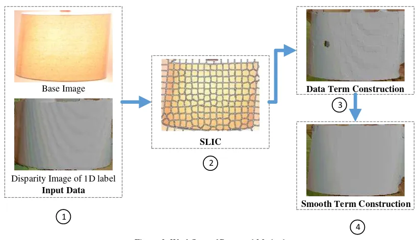
The work flow of GPM is shown in Figure 2. It consists of four parts: ○1E A The inputs of GPM are stereo pairs and the corresponding disparity image. A○2
E
A
SLIC (Achanta, et al., 2012) is adopted to segment the base image. A○3EA Construct data terms of patches one by one. The subfigure in A○3
E
A
presents the solution of energy function which only involves data terms. A○4EA Construct smoothness terms between patches. The subfigure in A○4
E
A
presents the solution of energy function which involves both data terms and smoothness terms. Finally, the disparity image with smooth surface can be obtained.
2.2 SLIC Segmentation
We assume that the scene is piecewise continuous and thus use SLIC to segment the base image into a series of patches. Every Patch can be described by a dispairty plane function:
�(�) = ��∙ ���+��∙ ���+��; � ∈ ��. (1)
where, Si represents the i th patch; ai, bi, ci represents the plane parameters of patch Si; �= (��,��)T represents a pixel in Si; (���,���)T represents centralized coordinates of �. The purpose of coordinate centralization is to improve the robustness of adjustment models.
Then, we check the number of valid disparities in each patch, because patches with little valid disparities are possible to be mismatches. The patches are called valid patches if they contain more valid disparities. Otherwise, the patches are called invalid
Input Data
Data Term Construction
SLIC
1
2
3
4
Base Image
Disparity Image of 1D label
Smooth Term Construction
disparities in patches are used to judge whether the patches are
2.3 Global Matrix Energy Function Construction
This paper defines matching as a global energy function. D
represents a disparity image. E(D) represents a global Energy function as follows:
�(�) =Edata+Esmooth. (3)
where, Edata represents a data term which measures the dissimilarity between a patch in the base image and the corresponding patch in the reference image; Esmooth represents a smoothness term which controls the smoothness between patches.
2.3.1 Data Term
Data term is defined as the summation of cost of all the valid patches, as follows:
�����=∑��=1�(��,���⃗ni). (4)
where, � represents the number of valid patches; C represents matching cost of patches; �� represents a patch; n���⃗i= (���,���,���)T represents the corrections of the disparity plane parameters in ��.
Correlation coefficients are defined as the matching cost in this paper. The matching cost of each patch in the base image is represents the initial disparity plane parameters which are computed from initial matching results; �i represents a patch in the base image; p represents a pixel in �i; �� represents the base image; �� represents the reference image; ����������(�i) represents the average intensity of all pixels in �i; �������������(�i|n���⃗i) represents the average intensity of all pixels in the corresponding patch of �i. �= (��,��) in the reference image represents the corresponding pixel of p; the coordinate�� can be obtained by the disparity plane function in Equation (1); the coordinate �� is equal to �� in the case of epipolar stereos.
Equation (5) shows that the correlation coefficient is a complicated nonlinear function. It is difficult to acquire the optimal solution of the global energy function in Equation (3), if the correlation coefficient in Equation (5) is adopted as the matching cost directly. It is worth noting that the correlation coefficient can be expressed as the second-order Taylor expansion, if good initial matching results are given.
�(�0+���,�0+���,�0+���|�� )
Equation (6) can be composed of matrices and vectors, as follows:
�(�0+��,�0+��,�0+��|�� )
where, �����(��) represents the quadratic coefficient matrix of the Taylor expansion for ��; �����(��) represents the linear coefficient matrix of the Taylor expansion for ��. The two coefficient matrices can be expressed as follows:
�����(��) is composed of unknowns of all the patches. The data term ����� can be expressed in the matrix form:
�����=���������� −2������ ��. (8)
Where, ����� represents the quadratic coefficient matrix of the data term; ����� represents the linear coefficient matrix of the data term. Constant term is neglected in Equation (8), because constant term has no influence on the computation of the optimal solution. All the coefficient matrices are expressed as follows:
�����=����(−�����(��))
�����= (−�����T (�1) −�T����(�2) ⋯ −�����T (��))�
Traditional least square feature matching methods introduce radiation correction parameters, which lead to a large unknown set. This paper proposes to use the the second-order Taylor expansion of the correlation coefficient as the matching cost, which can solve linear radiation distortion problems without introducing any radiation correction parameters. In the case of color image matching, the proposed GPM only use three unknowns for each patch, while traditional least square feature matching methods use nine unknowns for each patch. Besides, traditional correlation matching methods use fixed window, which will bring in fronto-parallel bias. The correlation window in this paper can be changed by disparity planes functions, which can remove fronto-parallel bias effectively.
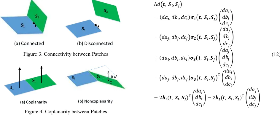
For any two adjacent patches, there are two geometrical relationships:
1. Connectivity Constraints. Any two adjacent patches are connected or disconnected, as shown in Figure 3. S1 and S2 represent adjacent patches. �= (��,��)T represents the border pixel in S1, which is adjacent to S2. Figure 3(a) shows the case that S1 and S2 are connected. Figure 3(b) shows the case that S1 and S2 are disconnected. This paper defines the connectivity measure as the distance from the border pixel to the plane of adjacent patches, as shown in Equation (9). CNCT(�, �1,�2) is small in the case of Figure 3(a), whereas it is large in the case of Figure 3(b). All the border pixels should be used to compute the connectivity measure.
CNCT��, ��,���=∆�(�, ��,��)
=������+�����+��− �����− �����− ���2 (9)
where, CNCT represents the connectivity measure between two adjacent patches; ∆� represents the square of disparity differences; (���,���) represents the centralized coordinates of border pixels in ��; (���, ���) represents the centralized coordinates of border pixels in ��; ��, ��, �� represent the disparity plane parameters of ��. ��, ��, �� can be expressed as the sum of initial parameters and the corresponding corrections, as follows:
��=�0+���,��=�0+���,�� =�0+���.
2. Coplanarity Constraints. The geometric relationship of any two connected patches is coplanar or noncoplanar, as shown in Figure 4. S1 and S2 represent two connected patches. c represents the centre of gravity in S2. Figure 4(a) shows the case that S1 and S2 are coplanar. The normal vectors of S1 and S2 in Figure 4(a) are parallel with each other. Figure 4(b) shows the case that S1 and S2 are noncoplanar. The most common way to measure the coplanarity of the connected patches is to compute the angle between normal vectors. However, the computation of the angle is a complicated nolinear function which will lead to high time complexity of correction computation. In order to avoid this problem, this paper defines the coplanarity of the connected patches as the distance from the center c to the plane of the adjacent patch, as shown in Equation (9). It can be seen from Figure 4(b) that S1 and S2 are more likely to be coplanar with
(a) Connected (b) Disconnected(b) Disconnected t
t tt
Figure 3. Connectivity between Patches
(a) Coplanarity
(a) Coplanarity (b) Noncoplanarity(b) Noncoplanarity S1
This paper defines smooth constraints as the combination of the connectivity constraints and the coplanarity constraints. This paper assumes that the surfaces of two adjacent patches are continuous smooth when the average intensity of the adjacent patches are close; otherwise, the smooth constraints are weak. The smoothness term ������ℎ can be defined as follows: coplanaritypenalty. The two penalties are defined as follows:
��1(�,�) =� ∙ ��� �− ���������� − ��(�i) ������������j� /��
��2(�,�) =��1(�,�)∙ ����<�i,�j>��
(11)
where, P represents a given penalty coefficient; � represents a smooth factor; ���<�i,�j> represents the angle between the normal vectors of �i and �j. ���<�i,�j> can be computed by the initial matching results. m represents a given power factor.
The first function in Equation (11) shows that when the average intensities of adjacent patches are close, a larger penalty ��1 should be given, which aims at encouraging smoothness in intensity homogenous regions. The second function in Equation (11) shows that a larger ��2 should be given, when the connectivity of the adjacent patches is strong and the angle between the normal vectors is small. A larger ��2 punishes
noncoplanarity of the adjacent patches. Otherwise, when the connectivity of the adjacent patches is weak or the angle between the normal vectors is big, smaller ��2 should be given to
guarantee the matching accuracy in curved areas.
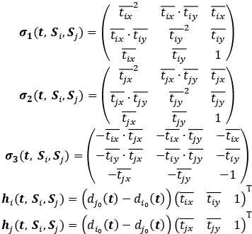
where, ��, ��, �� represents the quadratic coefficient matrices of ∆�, respectively; ��(�, ��,��) and ��(�, ��,��) represents the linear coefficient matrices of ∆�, respectively. Equation (12) neglects the constant term, which doesn't influence the computation of the optimal solution. The detailed expressions of ��, ��, ��, ��(�, ��,��) and ��(�, ��,��) are as follows: represents the disparity of pixel t, which is computed by the initial disparity plane parameters of �j.
The smoothness term ������ℎ can be rewritten in the matrix form by inserting Equation (12) into Equation (10).
������ℎ=������� −2����� (13)
where, �� represents the unknown vector composed of all the corrections of disparity plane parameters; �� represents the quadratic coefficient matrix of the smoothness term; �� represents the linear coefficient matrix of the smoothness term. The detailed description of �� is as follows:
The global energy function can be redefined in the matrix form by combining Equation (8) and Equation (13).
min�(�) =���(�����+��)�� −2(������ +���)��. (16)
Equation (16) is a typical objective function of least squares. Computing the minimum value of Equation (16) is equal to solving (�����+��)��=�����+��. There are many ways to acquire the optimal solution of Equation (16), such as conjugate gradient methods, quasi-newton method, Cholesky decomposition and so on. We used the Eigen tool to solve Equation (16) in all the following experiments.
3. EXPERIMENTS
In order to test the performance of the proposed method, two experiments were carried out. The Adirondack stereo and the Motorcycle stereo of Middlebury benchmark (Scharstein and Szeliski, 2002) are used as the experimental data We compared the performance of the proposed GPM with INTS (Huang, et al., 2016) which is one of the state-of-the-art 1D labels. Then, we used the ground truth to evaluate the matching accuracy of GPM. In both experiments, all the matching parameters were fixed. We used the INTS matching results as the initial matching of GPM in all the experiments.
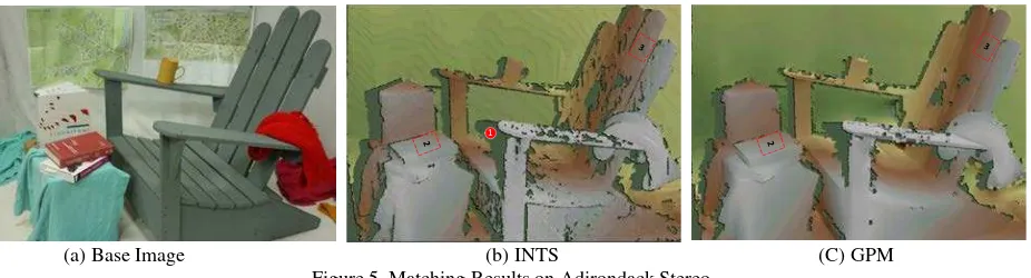
3.1 Experiment on Adirondack stereo
The base image of Adirondack is shown in Figure 5(a). Figure 5(b) is the disparity image generated by INTS. Figure 5(c) is the disparity image generated by the proposed GPM. Region 1 in Figure 5(b) represents invalid regions where disparities were invalid.
The reconstructed surfaces of INTS matching results face serious "disparity stair" problems, and the surfaces are rather rough, as shown in Figure 5(b). It is because 1D label algorithms assume fronto-parallel planes which can cause fronto-parallel bias. The proposed GPM can remove fronto-parallel bias. GPM assigns three labels to each patch and constructs smoothness terms between adjacent patches. Thus, the reconstructed surfaces of GPM matching results are continuous smooth, as shown in Figure 5(c). It is worth noting that the invalid pixels of GPM are much less than that of INTS in Figure 5. It is because not all of the disparities in each SLIC patch are valid, as descripted in section 2.2. Therefore, the optimal solution can be used to compute the disparity of invalid pixels in each valid patch, and a more complete disparity image can be obtained.
zoomed sight of Region 2 and Region 3 are illustrated in Figure 6 and Figure 7, respectively.
(a) INTS (b) GPM Figure 6. Comparison of Surface in Region 2
(a) INTS (b) GPM Figure 7. Comparison of Surface in Region 3
Figure 6 and Figure 7 show that the surfaces of GPM matching results are continuous smooth even in the zoomed sight. Ground truth was used to evaluate the performance of GPM. In order to give a comprehensive evaluation, this paper adopted the average matching accuracy, the percent of pixels with matching accuracy below 0.5 pixels, 1 pixel, 2 pixels and 3 pixels as accuracy metrics, respectively, as shown in Table 1.
Average (Pixel)
% < 0.5 Pixel
% < 1 Pixel
% < 2 Pixels
% < 3 Pixels
GPM 0.379 79.2 92.3 97.6 98.8
INTS 0.404 78.4 92.4 97.6 98.8
Iteration
Times 1
Table 1. Accuracy Evaluation of GPM on Adirondack Stereo
Table 1 shows that the matching accuracy of GPM is better than that of INTS. The matching accuracies of most pixels (79.2%) are below 0.5 pixels. The matching accuracies of almost all the pixels (98.8%) are below 3 pixels, which shows the good robustness of GPM. Smoothness terms make contributions to the robustness. It helps achieve the global optimal solutions. If no smoothness terms were used, GPM might trap in the local optimum, or even could not converge, which would lead to mismatches. The computation efficiency of GPM is high. Only one iteration was needed to obtain the continuous smooth surface model.
3.2 Experiment on Motorcycle stereo
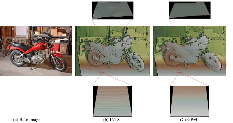
The base image of Motorcycle is shown in Figure 8(a). Figure 8(b) is the matching results of INTS. Figure 8(c) is the matching result of the proposed GPM.
1D label algorithms assume fronto-parallel planes, thus the surface of INTS matching results face serious "disparity stair" problems, as shown in Figure 8(b). The proposed GPM can remove fronto-parallel bias and acquire continuous smooth surfaces, as shown in Figure 8(c).
Though continuous smooth surfaces were obtained by GPM, excessive smoothness occurred in some regions. For example, Region 1 in Figure 8(a) and Figure 8(c) was over smooth. In Region 1, the disparities of the tyre and the disparities of the ground are discontinuous. However, the intensities of the tyre and the ground are close due to the shadow of the motorcycle. Therefore, GPM encouraged the disparities of the tyre and the ground to be continuous, which led to mismatches. The excessive smoothness showed that GPM performed weakly in regions with homogenous intensities but discontinuous disparities.
Ground truth was used to evaluate the performance of GPM. In order to give a comprehensive evaluation, this paper adopted the average matching accuracy, the percent of pixels with matching accuracy below 0.5 pixels, 1 pixel, 2 pixels and 3 pixels as accuracy metrics, respectively, as shown in Table 2.
Average (Pixel)
% < 0.5 Pixel
% < 1 Pixel
% < 2 Pixels
% < 3 Pixels
GPM 0.541 70.4 87.0 95.1 97.3
INTS 0.396 80.4 94.2 97.8 98.6
Iteration
Times 1
Table 2. Accuracy Evaluation of GPM on Motorcycle Stereo
The performance of GPM in Table 2 is still good with only one iteration. The average matching accuracy is 0.541 pixels. The matching accuracy of most pixels (70.4%) are below 0.5 pixels. However, the performance of GPM was worse than that of INTS. It is because there were some mismatches caused by excessive smoothness.
4. CONCLUSION
This paper proposed a novel global patch matching method to remove fronto-parallel bias and obtain continuous smooth surfaces. The main work of this paper were concluded as follows:
1 2
2 22
3
3 33
1. The second-order Taylor expansion of correlation coefficients was introduced into the matching cost computation for the first time. The expression of the second-order Taylor expansion only contains three unknowns. Compared with the traditional least square feature matching, the unknown set of the Taylor expansions is much smaller.
2. This paper defined the smoothness terms as the combination of the connectivity constraints and the coplanarity constraints, which is capable of guaranteeing the smoothness between adjacent patches.
3. This paper transformed stereo matching into the least square problem. The global energy function can be rephrasedin the form of a quadratic matrix function, which can be solved by the least square principle. .
Experiments on Adirondack stereo and Motorcycle stereo from Middlebury benchmark showed that the proposed GPM performed well in both stereos. Fronto-parallel bias can be removed effectively, and the reconstructed surfaces are continuous smooth. In future work, we will focus on solving the excessive smoothness problem.
ACKNOWLEDGEMENTS
This work was supported by the Chinese Parasol Entrepreneurial Partner Project of Wuhan Engineering Science & Technology Institute (Grant No. gkwt006).
REFERENCES
Achanta, R., Shaji, A., Smith, K., Lucchi, A., Fua, P., & Süsstrunk, S., 2012. SLIC Superpixels Compared to State-of-the-art Superpixel Methods. Pattern Analysis and Machine Intelligence IEEE Transactions on, 34(11), pp. 2274-2282.
Barnes, C., Shechtman, E., Finkelstein, A., et al., 2009. Patchmatch: a randomized correspondence algorithm for structural image editing. ACM Transactions on Graphics, 28(3), pp. 341-352.
Besse, F., Rother, C., Fitzgibbon, A., & Kautz, J., 2014. Pmbp: patchmatch belief propagation for correspondence field estimation. International Journal of Compuer Vision, 110(1), pp. 2-13.
Bleyer, M., & Gelautz, M., 2005. A layered stereo matching algorithm using image segmentation and global visibility constraints. ISPRS Journal of Photogrammetry and Remote Sensing, 59(3), pp. 128-150.
Bleyer, M., Rother, C., & Kohli, P., 2010. Surface stereo with soft segmentation. In: Computer Vision and Pattern Recognition, San Francisco, pp. 1570-1577.
Guney, F., & Geiger, A., 2015. Displets: Resolving stereo ambiguities using object knowledge. In: Computer Vision and Pattern Recognition, Boston, pp. 4165-4175.
Hirschmuller, H., 2008. Stereo Processing by Semiglobal Matching and Mutual Information. IEEE Transactions on Pattern Analysis and Machine Intelligence, 30(2), pp. 328-341.
Huang, X., Zhang, Y., Yue, Z., 2016. Image-guided Non-local Dense Matching with Three-Steps Optimization. In: ISPRS Annals of Photogrammetry, Remote Sensing and Spatial Information Sciences, Prague, pp. 67-74.
Klaus, A., Sormann, M., & Karner, K., 2006. Segment-Based Stereo Matching Using Belief Propagation and a Self-Adapting Dissimilarity Measure. In: International Conference on Image Processing, Hong Kong, pp. 15-18.
Kim, K. R., & Kim, C. S., 2016. Adaptive smoothness constraints for efficient stereo matching using texture and edge information. In: International Conference on Image Processing, Phoenix, pp. 3429-3434.
Kolmogorov, V., Zabih, R., 2001. Computing visual correspondence with occlusions using graph cuts. In: International Conference on Computer Vision, Vancouver, pp. 508-515.
Lempitsky, V., Rother, C., Roth, S., & Blake, A., 2009. Fusion moves for markov random field optimization. IEEE Transactions
1 1 1
1
on Pattern Analysis and Machine Intelligence, 32(8), pp. 1392-1405.
Li, L., Zhang, S., Yu, X., and Zhang, L., 2016. PMSC: PatchMatch-Based Superpixel Cut for Accurate Stereo Matching. IEEE Transactions on Circuits and Systems for Video Technology, PP(99), pp. 1-14.
Li, Y., Min, D., Brown, M. S., Do, M. N., & Lu, J., 2015. SPM-BP: Sped-Up PatchMatch Belief Propagation for Continuous MRFs. In: International Conference on Computer Vision, Santiago, pp. 4006-4014.
Olsson, C., Ulen, J., & Boykov, Y., 2013. In defense of 3d-label stereo. In: Computer Vision and Pattern Recognition, Portland, pp. 1730-1737.
Pham, C.C., Jeon, J.W., 2013. Domain transformation-based efficient cost aggregation for local stereo matching. IEEE Transactions on Circuits and Systems for Video Technology, 23(7), pp. 1119-1130.
Scharstein, D., Szeliski, R., 2002. A Taxonomy and Evaluation of Dense Two-Frame Stereo Correspondence Algorithms. International Journal of Computer Vision, 47(1), pp. 7-42.
Taniai, T., Matsushita, Y., & Naemura, T., 2014. Graph Cut Based Continuous Stereo Matching Using Locally Shared Labels. In: Computer Vision and Pattern Recognition, Columbus, pp.1613-1620.
Veldandi, M., Ukil, S., & Govindarao, K.A., 2014. Robust segment-based Stereo using Cost Aggregation. In: British Machine Vision Conference, Nottingham, pp. 1-11.
Xu, S., Zhang, F., He, X., et al., 2015. Pm-pm: patchmatch with potts model for object segmentation and stereo matching. IEEE Transactions on Image Processing, 24(7), pp. 2182-2196.
Yamaguchi, K., Hazan, T., Mcallester, D., & Urtasun, R., 2012. Continuous markov random fields for robust stereo estimation. Lecture Notes in Computer Science, 7576(1), pp. 45-58.