INTEGRATED QUALITY EVALUATION OF THE IN-SITU NETWORKING
MEASUREMENTS AND UPSCALING USING GAUSSIAN PROCESS REGRESSION
Gaofei Yin a, Ainong Li a, *
a Institute of Mountain Hazards and Environment, Chinese Academy of Sciences, Chengdu 610041, China
[email protected] (A. Li).
Commission IV, WG IV/3
KEY WORDS: In-situ Networking Observations, Upscaling, Quality Evaluation, Gaussian Process Regression, Uncertainty
ABSTRACT:
The flourished development of wireless sensor network technology sheds light to the effective and inexpensive collection of in-situ networking measurements. This will contribute to the temporal validation of coarse resolution remote sensing products. However, the quality evaluation of the in-situ networking measurements and upscaling is still problematic. This study proposed an evaluation method based on Gaussian Process Regression (GPR). Specifically, the qualities of networking measurements and upscaling were evaluated through the relevance of each plot, and the pixelwise coefficient of variation of the scaling results. Both of which can be generated by GPR. The preliminary results demonstrated the potential of the proposed method on quality evaluation of upscaling. Its potential on measurements (per se) quality evaluation will be analysed future.
* Corresponding author
1. INTRUDUCTION
Direct validation of coarse resolution remote sensing products need the support of in-situ measurements (Camacho et al., 2013; Fang et al., 2012; Yan et al., 2016). Moreover, an upscaling process is also needed to interpolate the discrete measurements and get a spatially explicit reference map (Morisette et al., 2006). Traditional in-situ measurements are often collected through field campaign which is often labor-intensive and time-consuming because of its manual nature (Breda, 2003; Jonckheere et al., 2004; Weiss et al., 2004). The flourished development of low-cost near-surface remote sensing sheds light to the effective and inexpensive collection of in-situ measurements (Campos-Taberner et al., 2016b; Ryu et al., 2014). Wireless sensor network (WSN) is one of near-surface remote sensing systems, which comprises an array of sensor nodes and a wireless communications system (Qu et al., 2014). The sensor nodes can be located according to site-specific spatial sampling strategies to capture the surface heterogeneity. Therefore, WSN can provide unattended networking observations, which are important for temporal validation.
Although the validation protocol has long been proposed (Morisette et al., 2006), a scientific question is still not clear: Is the reference map per se credible, and how to evaluate its credibility? For the in-situ networking observations from WSN, we should address an additional question: Is the automated, unattended observations accurate or robust enough to generate high resolution reference parameter maps.
The above scientific questions bring in the following main objective of this study: to propose an integrated framework to evaluate the quality of the in-situ networking observations and upscaling. The evaluation method is based on Gaussian Process Regression (GPR). Performances of the proposed method on the quality evaluation of upscaling were tested over a crop site. The in-situ networking observations and the corresponding high resolution NDVI were provided by the LAINet and the CACAO fused NDVI images, respectively. The evaluation of the LAINet observations through GPR is still in progress.
2. DATA COLLOCTION 2.1 LAINet observations
The research was conducted in a 5 km × 5 km region (centred at ~ 40°22′N, 115°46′E ) near Huailai, northern China (Figure. 1), which is one of core observation fields of the Validation network for Remote sensing Products in China (VRPC) (Ma et al., 2015). The selected size was tailored to match MODIS pixels.
Figure 1. Map of the study area overlaid by the MOD15A2 product pixels (nominal resolution of 1 km × 1 km). The displayed image corresponds to a color composite (bands 5-4-3) of Landsat-8 OLI image acquired on August 23, 2013. The points represent the locations of the plots in the LAINet observation system deployed in the study area.
field measurements. It can measure the leaf area index (LAI) automatically and continuously. LAINet consists of Below Node (BN), which is deployed below the canopy and records transmitted radiation, the Above Node (AN), which is used to record downward radiation above the canopy, and the Central Node (CN), which is used as a data reception and control node. Communication among the nodes is achieved through Zigbee protocol, while data exchange between the CN and the remote Data Server (DS) is completed through the General Packet Radio Service (GPRS) network.
The two types of measurement nodes (AN and BN) have the same hardware configuration and software functions to ensure their consistent response to radiation, which is the prerequisite to calculate gap fraction. Because the downward radiation above the canopy can be considered to be spatially homogeneous at local space, a small number of measurements can represent the 5 km × 5 km study area, so one AN was deployed, and the AN consists of three quantum sensors. The LAINet deployed in our study area contained 12 plots, and the locations of those plots were determined by the SMP (Sampling strategy based on Multi-temporal Prior knowledge) sampling approach (Zeng et al., 2015). SMP can capture the spatio-temporal variation of vegetation growth.
The LAI estimation algorithm is based on the gap fraction theory, and uses beam radiation at different solar zenith angles to measure multi-angle gap fraction. When calculating gap fraction in a certain solar zenith angle for each BN, the average of the measurements from the three quantum sensors equipped in the AN was taken as radiation reference (EA); meanwhile, the
average of the measurements from the nine quantum sensors equipped in the BN was taken as the transmitted radiation under the canopy (EB), and the ratio between them (EB/EA) was seen
as the gap fraction.
Our study period is between July 1 (DOY 182) and September 14 (257), 2013 when a LAINet observation system were deployed and operated in the study area. Due to the unexpected instrument failure (e.g., dead battery and communication failure) and weather condition (e.g., cloudy and rainy weather), not all measured LAINet values were valid. Therefore, the number of available field LAI measurements on each day is not the same (less than or equal to 12). In addition, the estimated LAI values from each plot were averaged over eight-days interval consistent with the compositing periods of MODIS eight-days LAI products. This averaging procedure reduces the random errors and facilitates the comparison to MOD15A2 LAI product. The eight-days composited measurements were hereafter denoted by the first day (in the form of Day Of Year, DOY) of the compositing period. The number of processed LAI measurement is 12, 12, 11, 10, 6, 8 and 8 on DOY 185, 193, 201, 209, 217, 225 and 233, respectively, with a total number of 67 during the study period.
2.2 NDVI data
Many vegetation indexes (VI) have been used to predict fine resolution LAI map. The normalized difference vegetation index (NDVI), which is one of the most utilized vegetation in LAI retrieval, was selected in this study.
Spatio-temporal matching between field measurements and NDVI maps must be ensured to reduce uncertainty caused by the spatial heterogeneity and the dynamics change of vegetation. To obtain fine-resolution NDVI maps with high enough
temporal sampling to match the field measurements from LAINet, the CACAO method (Verger et al., 2013) was used to blend frequent MODIS NDVI data with fine-resolution OLI NDVI data in our study area. See (Yin et al., 2017) for further details.
The NDVI value corresponding to each LAINet measurement was extracted from the fused NDVI images, according to the locations of the LAINet plots and the dates. In total, 67 NDVI-LAI pairs were established as the training dataset of the GPR model.
3. DESCRIPTION OF THE EVALUATION FRAMEWORK
GPR has been recently introduced as a powerful regression tool (Rasmussen and Williams, 2006). The model provides a probabilistic approach for learning the relationship between the input (NDVI, in this study) and output (reference LAI, in this study) with kernels. This model has been widely used in biophysical parameters retrieval (Campos-Taberner et al., 2016a; Verrelst et al., 2012a; Verrelst et al., 2012b).
In this section, we first review the general formulation of GPR for regression problems, then define its potential in the integrated quality evaluation of the in-situ networking observations and upscaling.
weight assigned to each one of them, and K is a kernel function evaluating the similarity between the test NDVI x and all N training NDVI. In this study, a scaled Gaussian kernel function was used,
spread of the relations for each dimension of the input, σn is the
noise standard deviation and ij is the Kronecher’s symbol.
Model hyperparameters θ = {v, σb, σn } and model weights αi can be automatically optimized by Type-II Maximum Likelihood, using the marginal likelihood (also called evidence) of the observations (LAINet measured LAI in this study).
For training purposes, we assume that the observed variable is formed by noisy observations of the true underlying function y=f(x)+ . Moreover we assume the noise to be additive independently identically Gaussian distributed with zero mean and variance σn. Let us define the stacked output values y = (y1,
2 *
* **
~
0,
f ( )
n
K
I
K
N
x
K
K
y
(3)
For prediction purposes, the GPR is obtained by computing the posterior distribution over the unknown output y*, p(y*|x*, D), where D = {xn, yn| n = 1, 2…N} is the training dataset, i.e., the
67 NDVI-LAI pairs in this study. Interestingly, this posterior can be shown to be a Gaussian distribution, p(y*|x*, D), = N (μ*,
σ*), for which one can estimate the predictive mean (point-wise predictions):
y
I
σ
K
K
μ
n1 -2 T
*
*
=
(
+
)
, (4)and the predictive variance (confidence intervals):
* 1 -2 T
* * *
*
=
K
-
K
(
K
+
σ
I
)
K
σ
n . (5)Note that the predictive mean is a linear combination of observations y, while the predictive variance only depends on input data and can be taken as the difference between the prior kernel and the information given by observations about the approximation function (Verrelst et al., 2012b).
The GPR model has potential to be readily applied to integrally evaluate the quality of the LAINet observations and upscaling, with the following two advantages. First, the obtained weights
αi gives the relevance of each plot (see Eq. (1)), and a plot with
a high weight means high credibility (can be used to evaluate the observation quality). Second, a GPR model can provide a pixelwise uncertainty level (see Eq. (5)) for the scaling LAI map (can be used to evaluate the upscaling quality).
4. PRELIMINARY RESULTS AND DISCUSSION In this section, we will show the potential of the GPR model on the evaluation of the upscaling results. The evaluation of the LAINet observations through GPR is in progress.
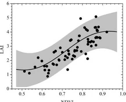
The regression result between the training NDVI-LAI pairs obtained using GPR and the predicted LAI values plus and minus twice the standard deviation (corresponding to the 95% confidence region) are shown in Figure 2. In terms of the uncertainty, several distinct regions can be easily observed. When NDVI < 0.5 or > 0.9, no training NDVI data are available, and the predicted LAI values have high uncertainty; when NDVI > 0.5 and < 0.9, where most of the training samples lie, the uncertainty in the predicted LAI values is relatively low. Therefore, the uncertainty given by GPR depends on the representativeness of the training dataset. Intuitively, the predicted value is credible if the GPR has ever seen the test value in the training phase. Otherwise, a high uncertainty will be returned if the test value is unfamiliar for the GPR.
Figure 2. Regression result of the training dataset using GPR. The shaded area represents the pointwise mean plus and minus twice the standard deviation for each NDVI value (corresponding to the 95% confidence region).
Although GPR can cope well with the strong nonlinearity of the functional dependence between the LAI and NDVI values, it displays a nonphysical trend. When the NDVI is very low, the LAI should approach zero. Second, the regressed curve should rise rapidly with the NDVI for high NDVI values, because of the saturation effect of the NDVI. However, the predicted LAI values level off when the NDVI is lower than 0.5 or higher than 0.9. This result is caused by the data-driven nature of GPR, and additional training samples with NDVI values lower than 0.5 or higher than 0.9 should be added to enhance the generalization ability of the trained GPR model. The limited sampling of the training dataset at low and high NDVI values would not lower the usability of the derived GPR model, because a high uncertainty is given for these specific NDVI values.
A point-by-point comparison between the observed LAI values from LAINet and the predicted LAI from GPR has also been implemented (Figure 3). In general, the GPR displays excellent accuracy, and the R2 and RMSE values of the GPR model are 0.72 and 0.45, respectively. GPR performed better than the empirical regression modeling approach implemented in a previous work (Yin et al., 2017), which resulted in an R2 value of 0.72 and an RMSE value of 0.55; see Fig. 7(b) in the paper cited above.
The time series of pixelwise LAI and uncertainty were generated and shown in Figure 4. Note that, to account for the dependence of variance on LAI value, the coefficient of variation (CV) rather than variance per se was used to represent the quality of the upscaling LAI. CV was calculated by
CV = (σ/μ)*100. (6)
The fine resolution LAI maps captured the vegetation dynamics well. At the beginning of the study period (DOY 185), crop near the water had smaller LAI (with LAI ranges from 1.0 to 2.0) than crop far from water (with LAI greater than 2.0) due to later sowing, and this caused obvious patchy pattern. After DOY 185, vegetation grew rapidly, and the spatial heterogeneity in the study area reduced. During DOY 209 to 225, vegetation reached growing peak with LAI exceeded 3.0 in most parts of the study area. Then, LAI decreased gradually. On DOY 233, most of the pixels had LAI of less than 3.0.
Besides the LAI time series, the GPR also generated the pixelwise CV time series, which indicate the quality of the resulting LAI. It can be seen from Figure 4 that the quality of the LAI maps also revealed an obvious temporal pattern, opposite to that of LAI series. On DOY 185, the LAI map showed a low quality, especially in northwest of our study area
where many pixels having CV greater than 50. After DOY 185, the quality of the upscaling LAI map continuously improved, Then after DOY 225, decreased again. In fact, the quality of the upscaling LAI inherits from the representativeness of the plots in LAINet. The SMP sampling strategy was designed to capture the spatio-temporal variation of vegetation growth and showed a good sampling efficiency (Zeng et al., 2015). But when implementing the SMP, the LAI was proxied by NDVI, SR and EVI (Zeng et al., 2015), which will show larger dynamic range in lower LAI value, because of the background disturbance. Therefore, VIs less sensitive to background influence should be used in future when determining the plot locations through SMP.
The temporal variation of the average LAI values and the uncertainty within our study area has also been analysed and is shown in Figure 5. Generally, these two variables show nearly symmetrical patterns, i.e., lower NDVI values are associated with higher uncertainties and vice versa. The negative correlation between the uncertainty and the NDVI values results from the under-sampling of the training dataset for low NDVI values (see Figure 2). Note that high NDVI values (>0.9) were also under-sampled, whereas the high NDVI values are not associated with large uncertainties. This result occurs because there are very few pixels that have an NDVI value higher than 0.9 in our study area.
Figure 4. High spatial resolution LAI maps and the corresponding quality evaluation results. The quality of each pixel is represented by its CV. Both LAI and CV were generated from the GPR model using LAINet measured LAI and CACAO reconstructed NDVI. The white parts represent non-vegetation land cover types.
Figure 5. The temporal variation of average LAI and uncertainty values in our study area.
5. CONCLUSIONS
networking observations per se will be conducted, and will be presented during the session.
ACKNOWLEDGEMENTS
This work was funded by the National Natural Science Foundation of China (41631180, 41601403, 41531174, 41571373) and the national key research and development program of China (2016YFA0600103).
REFERENCES
Breda, N.J.J., 2003. Ground-based measurements of leaf area index: a review of methods, instruments and current controversies. J Exp Bot 54, 2403-2417.
Camacho, F., Cemicharo, J., Lacaze, R., Baret, F., Weiss, M., 2013. GEOV1: LAI, FAPAR essential climate variables and FCOVER global time series capitalizing over existing products. Part 2: Validation and intercomparison with reference products. Remote Sens. Environ. 137, 310-329.
Campos-Taberner, M., Garcia-Haro, F.J., Camps-Valls, G., Grau-Muedra, G., Nutini, F., Crema, A., Boschetti, M., 2016a. Multitemporal and multiresolution leaf area index retrieval for operational local rice crop monitoring. Remote Sens. Environ. 187, 102-118.
Campos-Taberner, M., Javier Garcia-Haro, F., Confalonieri, R., Martinez, B., Moreno, A., Sanchez-Ruiz, S., Amparo Gilabert, M., Camacho, F., Boschetti, M., Busetto, L., 2016b. Multitemporal Monitoring of Plant Area Index in the Valencia Rice District with PocketLAI. Remote Sens. 8.
Fang, H.L., Wei, S.S., Liang, S.L., 2012. Validation of MODIS and CYCLOPES LAI products using global field measurement data. Remote Sens. Environ. 119, 43-54.
Jonckheere, I., Fleck, S., Nackaerts, K., Muys, B., Coppin, P., Weiss, M., Baret, F., 2004. Review of methods for in situ leaf area index determination - Part I. Theories, sensors and hemispherical photography. Agric. For. Meteorol. 121, 19-35. Ma, M., Che, T., Li, X., Xiao, Q., Zhao, K., Xin, X., 2015. A Prototype Network for Remote Sensing Validation in China. Remote Sens. 7, 5187-5202.
Morisette, J.T., Baret, F., Privette, J.L., Myneni, R.B., Nickeson, J.E., Garrigues, S., Shabanov, N.V., Weiss, M., Fernandes, R.A., Leblanc, S.G., Kalacska, M., Sanchez-Azofeifa, G.A., Chubey, M., Rivard, B., Stenberg, P., Rautiainen, M., Voipio, P., Manninen, T., Pilant, A.N., Lewis, T.E., Iiames, J.S., Colombo, R., Meroni, M., Busetto, L., Cohen, W.B., Turner, D.P., Warner, E.D., Petersen, G.W., Seufert, G., Cook, R., 2006. Validation of global moderate-resolution LAI products: A framework proposed within the CEOS Land Product Validation subgroup. IEEE Trans. Geosci. Remote Sens. 44, 1804-1817.
Qu, Y.H., Han, W.C., Fu, L.Z., Li, C.R., Song, J.L., Zhou, H.M., Bo, Y.C., Wang, J.D., 2014. LAINet - A wireless sensor network for coniferous forest leaf area index measurement: Design, algorithm and validation. Comput Electron Agr 108, 200-208.
Rasmussen, C.E., Williams, C.K., 2006. Gaussian processes for machine learning. the MIT Press 2, 4.
Ryu, Y., Lee, G., Jeon, S., Song, Y., Kimm, H., 2014. Monitoring multi-layer canopy spring phenology of temperate deciduous and evergreen forests using low-cost spectral sensors. Remote Sens. Environ. 149, 227-238.
Verger, A., Baret, F., Weiss, M., Kandasamy, S., Vermote, E., 2013. The CACAO method for smoothing, gap filling, and
characterizing seasonal anomalies in satellite time series. IEEE Trans. Geosci. Remote Sens. 51, 1963-1972.
Verrelst, J., Alonso, L., Camps-Valls, G., Delegido, J., Moreno, J., 2012a. Retrieval of vegetation biophysical parameters using Gaussian process techniques. Geoscience and Remote Sensing, IEEE Transactions on 50, 1832-1843.
Verrelst, J., Munoz, J., Alonso, L., Delegido, J., Rivera, J.P., Camps-Valls, G., Moreno, J., 2012b. Machine learning regression algorithms for biophysical parameter retrieval: Opportunities for Sentinel-2 and -3. Remote Sens. Environ. 118, 127-139.
Weiss, M., Baret, F., Smith, G.J., Jonckheere, I., Coppin, P., 2004. Review of methods for in situ leaf area index (LAI) determination Part II. Estimation of LAI, errors and sampling. Agric. For. Meteorol. 121, 37-53.
Yan, K., Park, T., Yan, G.J., Liu, Z., Yang, B., Chen, C., Nemani, R.R., Knyazikhin, Y., Myneni, R.B., 2016. Evaluation of MODIS LAI/FPAR Product Collection 6. Part 2: Validation and Intercomparison. Remote Sens. 8, 26.
Yin, G.F., Li, A.N., Jin, H.A., Zhao, W., Bian, J.H., Qu, Y.H., Zeng, Y.L., Xu, B.D., 2017. Derivation of temporally continuous LAI reference maps through combining the LAINet observation system with CACAO. Agric. For. Meteorol. 233, 209-221.