SHIFTS OF START AND END OF SEASON IN RESPONSE TO AIR TEMPERATURE
VARIATION BASED ON GIMMS DATASET IN HYRCANIAN FORESTS
KH. Kiapasha a, A.A. Darvishsefat a,*, N. Zargham a, Y. Julien b, J.A. Sobrino b, M. Nadic
a Dept. of Forestry and Forest Economics, Faculty of Natural Resources, University of Tehran, Karaj, Iran- ([email protected];
[email protected]; [email protected])
b Global Change Unit, Image Processing Laboratory, University of Valencia, P.O. Box 22085, E-46071 Valencia, Spain -
([email protected]; [email protected])
c Dept. of Irrigation, Faculty of Agricultural Engineering, Sari Agricultural Sciences and Natural Resources University-
KEY WORDS: Climate change, start of season, end of season, GIMMS NDVI3g, Hyrcanian forest.
ABSTRACT:
Climate change is one of the most important environmental challenges in the world and forest as a dynamic phenomenon is influenced by environmental changes. The Hyrcanian forests is a unique natural heritage of global importance and we need monitoring this region. The objective of this study was to detect start and end of season trends in Hyrcanian forests of Iran based on biweekly GIMMS (Global Inventory Modeling and Mapping Studies) NDVI3g in the period 1981-2012. In order to find response of vegetation activity to local temperature variations, we used air temperature provided from I.R. Iran Meteorological Organization (IRIMO). At the first step in order to remove the existing gap from the original time series, the iterative Interpolation for Data Reconstruction (IDR) model was applied to GIMMS and temperature dataset. Then we applied significant Mann Kendall testto determine significant trendfor each pixel of GIMMS and temperature datasets over the Hyrcanian forests. The results demonstrated that start and end of season (SOS & EOS respectively) derived from GIMMS3g NDVI time series increased by -0.16 and +0.41 days per year respectively. The trends derived from temperature time series indicated increasing trend in the whole of this region. Results of this study showed that global warming and its effect on growth and photosynthetic activity can increased the vegetation activity in our study area. Otherwise extension of the growing season, including an earlier start of the growing season, later autumn and higher rate of production increased NDVI value during the study period.
* Corresponding author
1. INTRODUCTION
The available data on climate change over the past century indicate that the Earth is warming (Khanduri et al., 2008). Climate change is one of the most important environmental challenges in the world and forest as a dynamic phenomenon is influenced by environmental changes. Changes in vegetation greenness over time may consist of an alternating sequence of greening and/or browning periods or shifts in start of season (SOS) and end of season (EOS).
Monitoring and attributing of vegetation dynamic is a prerequisite of sustainable management of ecosystem (Piao, et al., 2015). Trend analysis are one of the main research tools used to predict past and future states of the vegetation dynamic. Numerous studies of phenology and temperature has shown a widespread trend of advanced spring and later autumn of plants especially in the Northern Hemisphere have been documented, (Anyamba et al., 2005; Sherry et al., 2007; Julien et al., 2009; De Jong, et al., 2011; Hogda et al., 2013; Rodriguez-Galiano et al., 2015). We can find different trends in previous research because of various data sources, variable study periods, satellite platforms, temporal and spatial resolution from national to global scales.
As there is more than 40 years satellite records, the historic and long term records of satellite have become the most important source for monitoring of vegetation dynamics. Long term,
remotely sensed NDVI data as proxy of vegetation based on red/near infrared spectral, are suitable to detect and characterized trends of vegetation because it performed easily and closely related to vegetation productivity (Tian et al., 2015) which includes plants branches, stalks and leaves. NDVI time series have been widely used in trend analysis at regional to global scales. The longest continuous records of NDVI dataset provide by GIMMS group from Advanced Very High Resolution Radiometer (AVHRR) sensors onboard National Oceanic and Atmospheric Administration (NOAA) satellite series since July 1981. This dataset has been widely used for regional and global scale vegetation trend analysis representing changes in vegetation phenology (Anyamba et al., 2005; Baldi
et al., 2008; Julien et al., 2009; Sobrino et al., 2011). Furthermore, numerous international researches have focused on the relationship between variations of climatic variables such as rainfall and air temperature and changes in vegetation phenology (Ichii et al., 2002; Fensholt et al., 2011; Ivit et al.,
2012; Fensholt et al., 2013).
minimally during the entire Quaternary Era (Sagheb Talebi et al., 2014).
Many aspect of vegetation dynamics in Iran still remain poorly understood. Therefore, due to the importance of this ecosystem, this region deserves more attention to monitor the spatial patterns of vegetation dynamics and better characterization and discrimination of Hyrcanian forests are needed.
Therefore, with regards to importance of Hyrcanian forests in this study, we investigate the vegetation dynamics in Hyrcanian forests over 31-year period, based on GIMMS NDVI3g time series to analyze i: inter annual, ii: seasonal trend in vegetation dynamics. comprises a narrow strip of 1.8 million ha temperate deciduous forests and it contains very rich ecosystems due to the particular orographic and climatic situation (precipitation rich, warm-temperate, high moisture from the Caspian Sea and damming effect of the Alborz mountain range). The latitude and longitude of the Hyrcanian forests varies from 35˚ 45ˊ to 38˚ 26ˊ 15˝N and 38˚ 33ˊ 45˝ to 56˚ 11ˊ 15˝E, respectively (Fig. 1). In general, the Hyrcanian climate is warm Mediterranean in the east, and Mediterranean in the west (Sagheb Talebi et al., 2014). This area is one of the last remnants of natural deciduous forests in the world. The nomination of Hyrcanian forests as a UNESCO World Heritage site has been under attention since 2001 and have recently become one of the priorities of the Iranian government.
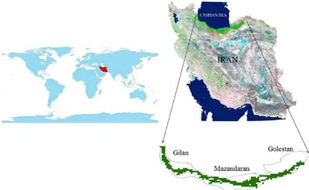
Figure 1: Geographical location of Iran (left) and of the Hyrcanian forests, extending over the Iranian provinces of
Guilan, Mazandaran and Golestan (right).
2.2 Data
The time series of GIMMS3g NDVI dataset with 0.083 degree spatial resolution and a temporal resolution of circa 15 days was used in this study. This dataset is derived from NOAA satellite series AVHRR instrument, spanning the period 1981-2012. In order to minimize the influence of atmospheric aerosols and clouds, the maximum value compositing (MCV) technique has been used to create composite images. Data have also been corrected to minimize various deleterious effects, such as inter sensor differences, viewing geometry, orbital drift and volcanic eruptions, and has been verified using stable desert control points (Pinzon et al., 2014). Validation of this dataset for
considering vegetation dynamic was considered in previous research (Zeng, et al., 2013; Miao et al., 2015).
In order to account effect of climatic warming on phenology, air temperature data recorded by 45 weather stations, fully covering the Hyrcanian area were used for correlation analysis. These data were provided by the Islamic Republic of Iran Meteorological Office and Iran Ministry of Energy. These point data were interpolated to the same resolution and geographic coordinate system as GIMMS3g NDVI dataset.
Forest boundaries were provided from Forests, Range and watershed Organization (FRO) of Iran and rasterized to the same spatial resolution as the GIMMS3g data. Since GIMMS has coarse pixel size (8 km × 8 km), it can include forest and non-forest and this research focused on forest areas, only pixels with more than 80 percent forest cover in compare with official vector map of forest were considered in the analysis (Fig. 1).
2.3 Methods
The analysis of raster data time series is based on a number of statistical techniques implemented in the statistical program R (R Development Core Team, 2008). First, in order to exclude remaining gaps caused by cloud or haze contamination which create low and discontinuous NDVI values in the time series, the iterative Interpolation for Data Reconstruction (IDR) method was applied pixel by pixel to GIMMS3g NDVI data. Based on previous researches (Julien & Sobrino, 2009; Geng et al., 2013), this method can provide the best profile reconstruction for most land cover classes. For each pixel, alternative NDVI time series was computed by computing the mean of the immediately preceding and following observation. This alternative value was then compared to the original time series, and replaced the original data with alternative time series data if the maximum difference between alternative and original values is higher than 0.02 NDVI units, corresponding to the accuracy of NDVI estimation (Julien & Sobrino, 2009; Sobrino, 2013; Kiapasha et al., 2017).
After this, start and end of season of every yearly seasonal time interval using the midpoint technique was calculated pixel by pixel for the study area. Midpoint technique is more consistent with the ground measured phenology than other methods (White et al., 2009; Wang et al., 2016). This technique first extracted minimum and maximum value for each pixel and individual year and determines the threshold value, and then the SOS is defined as the day of the year when 50 percent of the annual amplitude is reached through an increasing or decreasing in NDVI values (Julien et al., 2009; 2013; Kiapasha et al.,
2017). Increasing temperature influence vegetation phenology and NDVI time series respond to the climate change. In order to extract temperature parameters, all of these analyses were performed for temperature too. Five parameters were thus extracted (Table 1).
Label Parameter Unit
SOS Start of season Days
EOS End of season Days
Tempmean Mean of temperature ˚C
Tempmax Maximum of temperature ˚C
Tempmin Minimum of temperature ˚C
TempTmax Date of maximum temperature Days
Table 1: Extracted phenology and climate parameters using midpoint technique
The significance of the SOS and EOS time series trends were retrieved by the non-parametric Mann–Kendall (MK) significance test which has also a low sensitivity to outliers (Hirsch et al., 1984). Then we analyzed long time trend for temperature with the same spatial and temporal resolution of GIMMS dataset.
In order to compare the influence of climate parameters with different magnitudes, the first processing step is the normalization over parameters (temperature, SOS and EOS) by calculating their standardized anomalies according to (Ivit et al.,
2012; Kiapasha et al., 2017):
(1)
where z = resulting normalized value of parameters
xt = the original value = the mean value S = the standard deviation
The response of NDVI to temperature change was expressed as the linearly regressed slope of phenological parameter anomalies (SOS, EOS) against temperature anomalies for each pixel. This correlation was quantified using an ordinary least squares (OLS) regression. The regression equation was estimated as:
(2)
Where γ is the standardized anomaly of inter-annual variation of SOS and EOS, X1 is the standardized anomaly inter-annual variations of temperature, and � is the stochastic error term. In order to remove stochastic trend component (non-stationary) of time series, Time was used as a deterministic variable in the model.
3. RESULTS
In the following sections results are presented. We present phenological trends focusing on the SOS and EOS and their mapped correlation with changes of temperature.
3.1 Trend results
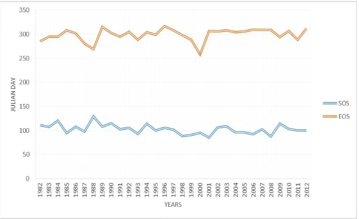
The SOS and EOS have been retrieved using the midpoint method over the period 1982 to 2012 for the Hyrcanian forests of Iran. They illustrate in figure 2.SOS and EOS derived from GIMMS3g NDVI time series increased by -0.16 and +0.41 days per year respectively. The statistically significant trends at 90% confidence level for the SOS and EOS for the period 1982– 2012 based on NDVI3g data are depicted in Figures 3 and 4.
Figure 2: Start and end of season from 1981 to 2012
Figure 3: Significant trends at 90% confidence level using Mann-Kendall trend test in start of season date (day/year)
SOS trends had non-significant values in most places and only few pixels with significant earlier SOS were scattered in Hyrcanian forests, whereas significant latter EOS appeared in most areas and a strong delay in EOS is observed for low altitudes.
EOS were more widespread than SOS trends and overall growing season lengthening for 1982-2012 may increasingly be
attributed to an EOS delay, This is close to the results of Garrona et al. (2016) and Jolly et al., (2005).
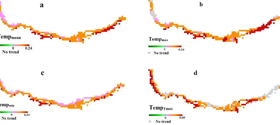
Figures. 5(a), (b), (c), and (d) shows the results of the pre-pixel trend analysis based on the anomaly of temperature parameters dataset. We observed no negative trends in temperature. Significant stronger positive trends were revealed in Golestan for Tempmean and Tempmax.
Figure 5: Significant trends at 90% confidence level using Mann Kendall trend tests in average of temperature (a), maximum temperature (b), minimum temperature (c), date of maximum temperature (d).
The current findings about temperature trends in this study confirm increasing air temperature as reported by IPCC (2013). Spatial distribution of the best multiple linear regression between inter annual variation of phenological parameters (SOS and EOS) and temperature parameters (Tempmean, Tempmax, Tempmin, TempTmax and TempTmin) calculated for each pixel in the Hyrcanian forests. Table 2 presents the percentage of pixels in the study showing significant (90 %) correlation SOS and EOS with each temperature parameters.
There were stronger correlations between SOS with Date of minimum and maximum temperature in most regions (30% and 24/5% of pixels, respectively) (Fig. 6(a), table 2), because SOS happen on the third month of year, thus value of temperature at the same year don’t influence SOS but spatially date of minimum temperature can be important, since minimum of temperature occur on January, February or March.
Stronger correlations between EOS and Tempmin than other temperature parameters were observed in 43% of pixels (Fig. 6(b), Table 2).
parameters EOS SOS
TempTmax 16 24/5
Tempmax 12.5 15
Tempmean 12.5 16/5
TempTmin 17 30
Tempmin 43 14/5
Table 2: Percentage of pixels with best linear regression with phenological parameters (EOS and SOS) as the dependent variable and the temperature parameters (TempTmax, Tempmax, Tempmean, TempTmin, Tempmin) as independent variables
Our findings illustrated strong correlations between later EOS and increasing temperatures mainly in western Hyrcanian forests.
Plant growth of the Hyrcanian forests is limited by temperature in high altitude. On the local scale other climatic and microclimatic variables might influence phenological changes better (Ivit et al., 2012), while the impact of anthropogenic activities on vegetation dynamics was not investigated. Hyrcanian forests consist various microclimates due to different slope direction, altitude and human activities that affect the response of phenological parameters in addition to climate factors. It should be mentioned that during the Pleistocene ("Ice Ages"), the Hyrcanian forests were alive and glaciations had minimal impact on it, and movement of some species to high altitude was imaginable (Sagheb Talebi et al., 2014) and could occur again, so biodiversity variation and vegetation dynamic should be monitored in this area to further observe global climate warming effects. Other climate variables such as precipitation, soil moisture, evapotranspiration or photoperiod can be related to variations in vegetation productivity.
Although many previous studies were carried out at the global or regional scales, these results cannot be easily compared with this research due to the geographical characteristics of the Hyrcanian forests, and to the spatial resolution of the dataset, leading to the relatively small number of pixels considered as forest in this study area.
4. CONCLUTION
Examining phenological trend in Hyrcanian forests over 1982-2012 reveals EOS trend was stronger than the SOS trend (EOS delay was 0.41 days yr-1, compared to -0.16 days yr-1 of SOS change). Later EOS trends were widely distributed over the Hyrcanian forests and significant trends in low altitude were observed in longer growing season.
The current findings about temperature trends in this study confirm increasing air temperature as reported by IPCC (2013). Moreover, EOS values were correlated positively and strongly with minimum temperature in 43 percent of pixels (Table 2) Important biological events, including changes in plant phenology, have been reported in many parts of the world (Khanduri et al., 2008), therefore we need more information information to attribute changes of our forest. This research is a first step to improve our knowledge of Hyrcanian forests by trend analysis of time series.
REFERENCES
Anyamba, A., Tucker, C.J., 2005. Analysis of Sahelian vegetation dynamics using NOAA-AVHRR NDVI data from 1981–2003. Journal of Arid Environments, Vol. 63, pp. 596– 614.
Baldi, G., Nosetto, M.D., Aragon, R., Aversa, F., Paruelo, J.M. and Jobbagy, E.G., 2008. Long-term Satellite NDVI Data Sets: Evaluating Their Ability to Detect Ecosystem Functional Changes in South America. Sensors, Vol. 8, pp. 5397-5425.
De Jong, R., De Bruin, S., De Wit, A., Schaepman, M. E., Dent, D. L., 2011. Analysis of monotonic greening and browning trends from global NDVI time-series. Remote Sensing of Environment, Vol. 115, pp. 692–702.
Fensholt, R., Rasmussen, K., 2011. Analysis of trends in the Sahelian ‘rain-use efficiency’ using GIMMS NDVI, RFE and GPCP rainfall data. Remote Sensing of Environment, Vol. 115, pp. 438–451.
Fensholt, R., Rasmussen, K., Kaspersen, P., Huber, S., Horion, S. and Swinnen, E., 2013. Assessing Land Degradation/Recovery in the African Sahel from Long-Term Earth Observation Based Primary Productivity and Precipitation Relationships. Remote Sensing, Vol. 5, pp. 664-686.
Garrona, I., De Jong, R. De Wit, A.J.W., Mucher, C.A., Schmid, B. and Schaepman, M.E., 2015. Strong contribution of autumn phenology to changes in satellite-derived growing season length estimates across Europe (1982–2011). Global change biology, Vol. 20, pp. 3457–3470, doi: 10.1111/gcb.12625
Hirsch, R.M. and Slack, J.R., 1984. A nonparametric trend test for seasonal data with serial dependence. Water Resources Res., vol. 20, pp. 727–732.
Hogda, K.A., Tommervik H. and Karlsen, S.R., 2013. Trends in the Start of the Growing Season in Fennoscandia 1982–2011.
Remote Sens. Vol. 5, pp. 4304-4318.
Ichii, K., Kawabata, A. and Yamagichi, Y., 2002. Global correlation analysis for NDVI and climatic variables and NDVI trends: 1982–1990. International Journal of Remote Sensing, Vol. 23, No. 18, pp. 3873–3878.
IPCC, Climate Change 2013: The Physical Science Basis, Contribution of Working Group I to the Fifth Assessment Report of the Intergovernmental Panel on Climate Change, T.F. Stocker, D. Qin, G.-K. Plattner, M. Tignor, S. K. Allen, J. Boschung, A. Nauels, Y. Xia, V. Bex and P.M. Midgley (eds.)]. Cambridge University Press, Cambridge, United Kingdom and New York, NY, USA, 1535pp, 2013.
Ivit, E., Cherlet, M., Toth, G., Sommer, S., Mehl, W., Vogt, J., Micale, F., 2012. Combination satellite derived phenology with climate data for climate change impact assessment. Global and planetary change, pp. 85-97.
Jolly, W.M., Nemani, R., and Running, S.W., 2005. A generalized, bioclimatic index to predict foliar phenology in response to climate. Global Change Biology, Vol. 11, pp. 619– 632.
Julien, Y., and Sobrino, J.A., 2009. Global land surface phenology trends from GIMMS database. International Journal of Remote Sensing, vol. 30, no. 13, pp. 3495–3513.
Khanduri, V.P., Sharma, C.M., Singh, S.P., 2008. The effects of climate change on plant phenology. The Environmentalist 28(2):143-147
Kiapasha, Kh., Darvishsefat, A.A., Julien, Y., Sobrino, J.A., Zargham, N., Atarod, P., Schaepman, M., 2017. Trends in phenological parameters and relationship between land surface phenology and climate data in the Hyrcanian Forests of Iran.
Miao, L., Liu, Q., Fraser, R., Bin He a, Cui, X., 2015. Shifts in vegetation growth in response to multiple factors on the Mongolian Plateau from 1982 to 2011. Physics and Chemistry of the Earth, Vol. 87-88, pp.50-59.
Piao, Sh., Yin, G., Tan, J., Cheng, L., Huang, M., Li, Y., Liu, R., Mao, J., Myneni, R.B., Peng, Sh., Poulter, B., Shi, X., Xiao, Zh., Zeng, N., Zeng, Zh., Wang, Y., 2015. Detection and attribution of vegetation greening trend in China over the last 30 years. Global Change Biology, 21, 1601–1609, doi: 10.1111/gcb.12795
Pinzon, J.E., and Tucker, C.J., 2014. A Non-Stationary 1981– 2012 AVHRR NDVI3g Time Series. Remote Sensing. Vol. 6, pp. 6929-6960.
R Development Core Team, 2008. R: a Language and Environment for Statistical Computing. R Foundation for Statistical Computing, Vienna, Austria. http:// www.R-project.org.
Rodriguez-Galiano, V.F., Dash J. and Atkinson, P.M., 2015. Characterizing the Land Surface Phenology of Europe Using Decadal MERIS Data. Remote Sens., vol. 7, pp. 9390-9409.
Sagheb Talebi, Kh., Sajedi, T., Pourhashemi, M., 2014. Forests of Iran ‘A Treasure from the Past, a Hope for the Future.
Sherry, R.A., Zhou, X., Gu, Sh., Arnone, J.A., Schimel, D.S., Verburg, P.S., Wallace, L.L., and Luo, Y., 2007. Divergence of reproductive phenology under climate warming. Proceeding of the National academy of Science of the United States of America (PNAS), Vol. 104, No. 1, pp. 198–202.
Sobrino, J.A., Julien Y. and Morales, L., 2011. Changes in vegetation spring dates in the second half of the twentieth Century. International Journal of Remote Sensing, iFirst, pp. 1– 18.
Sobrino, J.A., Julien, Y. and Soria, G., 2013. Phenology Estimation From Meteosat Second Generation Data. IEEE Journal of selected topics in applied earth observations and Remote Sensing, Vol. 6, NO. 3, pp. 1653- 1659.
Tian, F., Fensholt, R., Verbesselt, J., Grogan, K., Horion, S., Wang, Y., 2015. Evaluating temporal consistency of long-term global NDVI datasets for trend analysis. Remote Sensing of Environment, Vol. 163, pp. 326–340.
Wang, S., Yang, B., Yang, Q., Lu, L., Wang, X., Peng, Y., 2016. Temporal Trends and Spatial Variability of Vegetation Phenology over the Northern Hemisphere during 1982-2012.
PLoS ONE 11(6): e0157134.
https://doi.org/10.1371/journal.pone.0157134
White, M.A., De Beurs, K.M., Didan, K., Inoy, D.W., Richardson, E.A.D., Jensen, O.P., Keefe, J.O., Zhang, G., Nemani, R.R., Leeuwen, W.J.D.V., Brown, J.F., De Wit, A., Schaepman, M., Lin, X., Dettinger, M., Bailey, A.S., Kimball, J., Schwartz, M.D., Baldocchi, D.D., Lee, J.T., Lauenroth, W.K., 2009. Intercomparison, interpretation, and assessment of spring phenology in North America estimated from remote sensing for 1982–2006. Global Change Biology, pp. 1365-2486.