AN EFFICIENT METHOD TO DETECT MUTUAL OVERLAP OF A LARGE SET OF
UNORDERED IMAGES FOR STRUCTURE-FROM-MOTION
X. Wang a *, Z.Q. Zhan b, C. Heipke a
a Institute of Photogrammetry and GeoInformation, Leibniz Universität Hannover, Germany – (wang, heipke)@ipi.uni-hannover.de b School of Geodesy and Geomatics, Wuhan University, 129 Luoyu Road, Wuhan 430072, People’s Republic of
KEY WORDS: unordered set of images, image orientation, random k-d forest
ABSTRACT:
Recently, low-cost 3D reconstruction based on images has become a popular focus of photogrammetry and computer vision research. Methods which can handle an arbitrary geometric setup of a large number of unordered and convergent images are of particular interest. However, determining the mutual overlap poses a considerable challenge.
We propose a new method which was inspired by and improves upon methods employing random k-d forests for this task. Specifically, we first derive features from the images and then a random k-d forest is used to find the nearest neighbours in feature space. Subsequently, the degree of similarity between individual images, the image overlaps and thus images belonging to a common block are calculated as input to a structure-from-motion (sfm) pipeline. In our experiments we show the general applicability of the new method and compare it with other methods by analyzing the time efficiency. Orientations and 3D reconstructions were successfully conducted with our overlap graphs by sfm. The results show a speed-up of a factor of 80 compared to conventional pairwise matching, and of 8 and 2 compared to the VocMatch approach using 1 and 4 CPU, respectively.
* Corresponding author
1. INTRODUCTION
In close-range photogrammetry untrained users typically do not record images in a pre-planned pattern, and even experts often need significantly more time for data acquisition when strict recording protocols must be followed. For some years, following the development of sensor and electronic information technology, users can obtain plenty of images of interesting objects using mobile phones, digital cameras or from the Inter-net (Snavely et al., 2008a). How to compute 3D information in an efficient way from this set of unordered images has become an vivid research and development topic (Agarwal et al., 2009, Frahm et al., 2010). In this context “unordered” means that there is no prior knowledge of which images have a common field of view (overlap) and should be matched.
For automatic image orientation and 3D reconstruction, a large number of high-dimensional features (using e.g. the scale-inva-riant feature transform (SIFT, Lowe, 2004) are generally extracted from images which then need to be matched before computing 3D points. For unordered images, where it is not known which images share a common field of view and should therefore be matched, the two most time-consuming subtasks are feature matching and bundle adjustment. This paper is dedicated to feature matching. A naive exhaustive pairwise matching procedure imposes a significant computational burden on large-scale 3D reconstruction. Nevertheless, some state-of-the-art approaches such as the well-known 3D modelling sys-tem Photo Tourism (Snavely et al., 2008a) derive overlapping image pairs by exhaustive pairwise image matching, needing N*(N-1)/2 matchings, where N is the number of images. This strategy can become unacceptable if the dataset to be processed contains a very large number of images.
This paper proposes an improved strategy based on a random k-d forest. After the rank-dom k-k-d forest is built, the methok-d is
linear in N. The main contribution is threefold: First, we show that several independent random k-d trees (a random k-d forest) can be built from the extracted SIFT points by setting different splitting hyperplanes, and that the k nearest neighbour points of a point being queried can be retrieved efficiently. Second, an algorithm is introduced to determine the degrees of similarity and the image overlaps of the unordered images by using the results of the random k-d forest, and we propose an algorithm to eliminate gross errors from the image overlaps by clustering and discarding single images. Finally, the overlap results are integrated into a general structure-from-motion (sfm) pipeline, where only the overlapping image pairs are considered.
2. RELATED WORK
As mentioned before, in sfm matching images is one of the most time-consuming processes. A naive approach needs N*(N -1)/2 matchings to find tie-points if no prior knowledge of the image orientations is available. Suggestions to speed up this method exist, of course.
stricter criteria for feature selection. When usingachieved using classical image pyramids (e.g. Mayer 2003; Wu, 2013) or by stricter criteria for feature selection. When using SIFT for feature extraction, setting a stricter Difference-of-Gaussians (DoG) threshold can achieve the goal; see e.g. VLFeat (Vedaldi and Fulkerson, 2008). However, this reduction can lead to the elimination of features which are important for computing the orientation, and it is then possible that the sfm computation fails altogether. To overcome this problem, supervised classification schemes were proposed to differentiate between matchable features (i.e. those for which a conjugate partner exists in another image) and unmatchable ones. Supervised classification needs training data. Hartmann et al. (2014), who use random forests for the classification, chose some sample images to be matched by ANN for training. The trained random forest was then considered as a predictor to decide which feature is matchable and to discard those features which are not matchable. It was found that random forests can discard many unmatchable features, but only if the training samples are representative enough for the whole image dataset. Moreover, a considerable amount of time is required to generate the training data if the number of sample images is large.
Yet another method called vocabulary tree, first introduced by Nistér and Stewenius (2006), is based on the assumption that across all images homologous features should be similar. This observation is exploited by quantising the feature descriptors and then finding other images, e.g. stored in a database, with many similar descriptors. Typically tree structures are used for retrieval, and the k-means algorithm is employed to find the k closed neighbours. The process can be carried out hierarchically until a pre-specified level of detail is reached; in this way a tree, the vocabulary tree, is created. Each cluster of the vocabulary tree is regarded as one word. It is intuitive that the matchable points should be classified into the same word and unmatchable points should be in different words (Farenzena et al., 2009). To calculate the degree of similarity between images, the so called term frequency inverse document frequency (tf-idf) is used to generate image weights. These weights ensure that words appearing seldom have a larger weight (Sivic and Zisserman, 2003). Although the method works well, k-means needs several iterations to determine each cluster centre. Thus, it can become very inefficient to cluster so many features from a large set of unordered images. Also, some clusters will contain un-matchable points if the number of features (from all images) is larger than the number of clusters of the last level: this may hamper the following steps.
To improve the efficiency of the vocabulary tree and decrease the mentioned negative influence Zhan et al. (2015) proposed a multi-vocabulary tree implemented of a graphics processing unit (GPU). Different vocabulary trees are built and each word is evaluated by computing the average value of the distance between each feature to its cluster centre. The authors show that efficiency and precision are improved, but, the method is limited by the performance of the GPU, and also in the multi-vocabulary tree a number of unmatchable features exists, which enter and thus slow down the computations.
To avoid mixed clusters, i.e. clusters containing matchable and unmatchable points, the number of clusters is significantly in-creased in a method named VocMatch (Havlena and Schindler, 2014). The authors propose a 2-level vocabulary tree, the first level with 4096 clusters, and the second level with 4096* 4096 clusters. All features of all images are contained in the resulting about 16 million words. It is assumed that the features which
are clustered into the same word in the second level are matchable points. Again, rare words are preferred. Obviously, a considerable amount of time is needed to compute the 4096* 4096 clusters. To make the algorithm more efficient, the authors use a pre-training procedure for the clusters of both levels, the results of which are assumed to be valid for different datasets. Whether or not this assumption is valid remains unclear.
Graph optimization methods were also proposed to speed up the sfm process. Skeletal graphs for efficient sfm were designed to compute a small subset of images. Snavely et al. (2008b) reconstruct the skeletal set and then add the remaining images using pose estimation. In Havlena et al. (2010), the so called approximate minimal connected dominating set of images was computed using a fast polynomial algorithm. Those two methods are proposed for fast image orientation. They are not applicable, however, without image overlap information. Approximate methods which iteratively build the skeletal graph (Agarwal et al., 2009) have been suggested for this issue.
The above mentioned works try to determine the mutual overlap of unordered images taken from different views. We are in-spired by the vocabulary tree method which clusters the high-dimensional features in feature space (we use the SIFT feature detector and thus deal with 128 dimensions). But, instead of the hierarchical k-means algorithm, which needs a lot of computing effort, a random k-d forest is used for clustering. In this way, each feature’s k nearest neighbours can be obtained by traversing the generated random k-d forest, and so can the distances between a feature and its nearest neighbours. Further-more, we propose an algorithm to compute the degree of similarity of images and we eliminate single images which may result from wrong nearest neighbours.
3.1 Building the random k-d forest
The k-d tree is a form of balanced binary search tree (Robinson, 1984) and has been widely used in conducting nearest neighbour queries for image descriptors. For low dimensional data, the k-d tree gives good results, in both efficiency and precision. As an example, Arya et al. (1998) proposed the so called priority search algorithm, a method which is based on a k-d tree and which can quickly complete a nearest neighbour search in low dimensions. However, when dealing with high dimensional data, a very large number of nodes may need to be searched, and when faced with a large amount of data, there will be a lot of backtracking, which reduces the retrieval efficiency. We propose an improved method for calculating the similarity degrees and image overlaps of a large set of unordered images based on a random k-d forest. To build the random k-d forest, we follow the following rules:
1) To make the k-d trees of the forest independent of each other, each k-d tree should have a different tree structure. 2) Priority search is applied in each k-d tree. To improve the
candidates will be obtained after the search is complete. Among these m*n nearest candidates, the r nearest candidates are then selected.
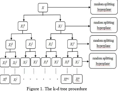
Figure 1. The k-d tree procedure
As Fig. 1 shows, the original data are recursively split into two nodes by a splitting hyperplane. When dealing with k-d trees, typically the entry of the high-dimensional feature with the largest variance is chosen for splitting. In order to make the trees more independent we instead select the splitting plane randomly from a range of entries with relatively large variances, and we randomly select the hyperplane anew for every splitting operation. All k-d trees are built using this same algorithm.
3.2 Determining the similarity degree and overlap between images
According to the above algorithm, the random k-d forest is built by employing all SIFT features from all unordered images. In this way each SIFT feature point obtains r nearest neighbour points and the distances between the query point and these neighbour points. The similarity degrees and the overlap of the unordered images can then be determined. The specific processes are as follows:
1) Obtain the r nearest neighbour points of each SIFT feature point from the i-th image (i=1,2, 3, … , N) by traversing the random k-d forest, where N is the number of unordered images. We then select the l nearest neighbouring images for the i-th image, i.e. one per tree of the forest. The number of the resulting neighbours per image pair ij is called Pij, where j is the image ID of j-th image.
2) By adding up the distances between the SIFT feature points of the i-th image and their neighbours, we obtain a distance measure Dij, where j is again the image ID of j-th image. 3) The larger the value of Pij, the more potential matches
between the i-th and j-th image exist, and the more likely it is that the two images overlap. According to our experience, Pij should be larger than 20. Furthermore, the smaller the value of Dij, the more similar the two images are. We then calculate the so called degree of similaritySij between the i-th and j-th image, equation (1): the more
Among the set of unordered images, we determine this degree of similarity from all potential image pairs; this information
reduces the computational effort for subsequent pairwise matching to a large extent, as we only undertake matching for similar images.
Based on Sij one simple way to determine the image overlap is to choose, for each image, the images with the f largest Sij values. Typically, such a procedure will only produce approximate overlap information. In an attempt to obtain more accurate results, Zhan et al. (2015) proposed a method which performs well in removing wrong overlaps. It assumes that the number of overlapping images (which we call the overlap degree C) is at least approximately known. The main steps are as follows:
1) We first take the C partners of a given image with the highest S values and compute the average and the standard deviation of the similarity values.
2) For any additional images, if the absolute difference between the similarity value and the average is smaller than twice the standard deviation, the new image is considered to also be overlapping with the image under investigation, and we recalculate average and standard deviation of the enlarged set of images. Otherwise, the new image is assumed not to overlap with the image under consideration, and we discard it.
3.3 Clustering unordered images and discarding single images
Typically, large sets of unordered images, especially crowd-sourced images collected from websites, naturally decompose into several smaller unconnected clusters (i.e. there are no or not enough tie-points between different clusters). Moreover, there sometimes exist single images which are not connected to any of the other images.
Algorithm 1 Clustering images and discarding single images Input Symmetric N*N matrix Q.
have a minimum of cpmin conjugate points (we use a threshold of 30) and delete the connection otherwise. Subsequently, an adjacency matrix A is derived (see Algorithm 1 for details) that determines which images have enough conjugate points to be a part of the same cluster. By traversing each image in A, we obtain the different clusters. Clusters which have less images than a pre-defined threshold (we empirically found that 50 works well) are considered as unreliable and are discarded.
4. EXPERIMENTS
All experiments are carried out using real data. The data consist of three different groups of images: the first one is made up of two different clusters, 301 UAV images of an urban area from Wuhan, China, and 296 close range images showing a relic of Xinjiang province also in China (see the right part of Fig. 4(a)); the second group contains 450 images of the main building of Hannover University, some acquired on a sunny day, some on a cloudy day (Fig. 4(b)). The last group is the Notre Dame dataset (Snavely, 2016) containing 715 images (Fig. 4(c)). According to preliminary experiments, the overlap degree C is set to 20.
4.1 Overlap results of unordered images
(a) (b)
Figure 2. The result for the first image group: (a) similarity graph, (b) overlap graph (see text for details)
Based on the proposed method, the degrees of similarity and overlap of the first group were calculated. Fig. 2(a) shows the similarity graph, i.e. the results computed with eq. (1), Fig. 2(b) depicts the overlap graph, i.e. the result after applying the method of Zhan et al. (2015) described at the end of section 3.2. For both figures the horizontal and vertical axes are the image IDs from 1 to 597 (which is the size of the data set). White means that the two corresponding images have a high similarity or overlap, black stands for a low similarity or overlap. The white dots mostly lie along the main diagonal, which tells us that the numbering scheme of the images reflects the sequence of acquisition. It can be seen in Fig. 2(b) that the group consists of two different clusters. Accordingly, our method correctly divides the group into two clusters, see Fig. 3(a) and 3(b).
(a) (b)
Figure 3. The sub-cluster overlap graphs of the first image graph
4.2 SFM results
We have applied our approach to the other two unordered image groups as well. To demonstrate that the results are qualitatively correct, the three unordered image groups (the first one in two sub-groups) were orientated and coarse 3D recon-structions were produced by sfm. Specifically, the unknown image overlaps were calculated by our algorithm, and only overlapping image pairs were considered for matching. A few software packages, e.g. VisualSFM (Wu, 2016) and COLMAP (Schönberger, 2016), can use this overlap information instead of carrying out exhaustive pairwise image matching. We used VisualSFM.
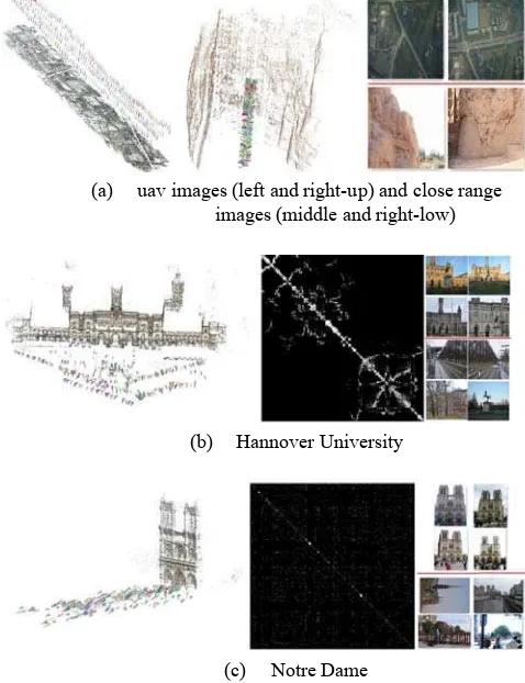
(a) uav images (left and right-up) and close range images (middle and right-low)
(b) Hannover University
(c) Notre Dame
Figure 4. SFM results of three experimental image groups
Fig. 4 depicts the result, coarse 3D reconstructions of the three experimental image groups, together with the similarity graph and a few sample images. As many off-diagonal elements of the similarity graphs are white, image acquisition in the second case occurred more ad hoc, and even random for Notre Dame. Images above the horizontal red bar of the right part of Fig. 4(b) and (c) are classified into clusters that contain more than 50 images and are used for sfm. Images below the bar are single images or images belonging to small size clusters which are discarded by our approach.
4.3 Analysis of the time efficiency
Number of image
Proposed method, 1 CPU Exhaustive pairwise matching
VocMatch Calculating
overlap
graph Matching Total 1 CPU 4 CPUs
301 UAV images and
296 close range image
597 4min42sec 12min12sec 16min54sec 848min (50×) 106min (6.8×) 29min (1.7×)
Main building of
Hannover University
450 3min53sec 10min36sec 14min29sec 482min (33×) 86min (6×) 24min (1.7×)
Notre Dame 715 5min35sec 9min34sec 15min9sec 1217min (81×) 127min (8.5×) 35min (2.3×) Table 1. Computational time needed for three methods for processing the three data sets. In our method, matching refers to the generation of conjugate points in image space. The numbers in brackets below the times of the Exhaustive pairwise match and
VocMatch refer to the achieved speedup factor of our method. All timings are based on the mentioned hardware setup. All experiments were conducted under the QT platform and the
system environment of VS2015 and OpenCV. In all experi-ments the result are the image coordinates of conjugate points in image space, image orientation and coarse 3D reconstruction are not considered in the timings given.
The system hardware configuration was an Intel Core i5 CPU, and the graphics card was a HD Graphics 530. A state-of-the-art CUDA-enabled SiftGPU matching from VisualSFM was used in exhaustive pairwise matching and in the matching part of our method. The graphics card was not used in VocMatch and in our generation of the overlap graph. The code used for VocMatch is the one available at Havlena, Schindler (2016), it is tested for one and four CPUs.
For our method we individually specify the times for calculating the overlap graph and for matching. It can be seen that the matching, although performed using parts of the VisualSFM and thus the graphics card, takes considerably more time than the generation of the overlap graph, i.e. our main result. Although the number of Notre Dame images is the largest, the matching time is the shortest. The reason is that there are fewer actually overlapping images, which can also be seen in Fig. 4(b) and (c).
Tab.1 further (and not surprisingly) illustrates that, as the number of images grows, so does the computing time. For exhaustive pairwise matching the computation time increases by nearly a factor of 3 when comparing the second group (450 images) and the last one (715 images). For VocMatch the factor is about 1,5; whereas for our method it is only 1,3 (overlap computation) or 1,05 (overlap and matching).
Finally, our proposed approach is 50×, 33×, 81× faster than the exhaustive pairwise matching, respectively, for the three datasets. By building a 2-layer vocabulary tree, VocMatch does improve the efficiency, but depending on the number of non-empty clusters for each quantised SIFT feature VocMatch must compute up to 4096*4096 distance computations between two 128-dimension vectors in the second level; up to 4096*4096*n computations are required for n SIFT points. Compared to VocMatch, building k random k-d trees for the proposed method needs k*n*log2n distance computations for selecting the splitting hyperplanes. From Tab. 1, our approach with only one CPU is about 6 to 8.5 times faster than 1-CPU VocMatch. The more CPUs VocMatch uses, the higher the efficiency is, for
instance, with 4 CPUs for VocMatch our method is only slightly (about 2 times) faster.
4.3.2 Time efficiency of different size random k-d forests: We now analyse the effect of the number of trees in the random k-d forest (note that the effect of the number of trees on the correctness of the result is analysed in section 4.4). We test four relatively small random k-d forests, each with datasets of different size (5 to 70 images) from Notre Dame. Fig. 5 depicts the results. As can be seen the more k-d trees the random k-d forest has, the more time it needs to construct the overlap between the unordered images. Moreover, nearest neighbours must be searched for on each tree of the random k-d forest. In the investigated example we obtain a rather linear relationship: the time of 10 k-d trees is about 2.5 times that of 4 k-d trees. Similarly, with 4 k-d trees the method is twice as fast as with 8 k-d trees, and compared to a 6 k-d trees the method is almost 1.5 times faster with 4 k-d trees.
Figure 5. Computational time for random k-d forest with different sizes.
4.4 Evaluation of the overlap of the unordered images In the work of Davis and Goadrish (2006), the precision-recall and receiver operating characteristic (ROC) curves are introduced to present results for binary decision problems. Here, we use the criteria for assessing the quality of our results. A generic confusion matrix is shown in Tab. 2, and the connection between the entries of the confusion matrix and those of the ROC curve are given in equation (2).
To obtain a first impression of the confusion matrix resulting from our method, we tested a set of 120 UAV images by
Actual positive Actual negative
Predicted positive TP FP
Predicted negative FN TN
Re
Pr
TP
call True Positive Rate
TP FN
TP FP
ecision False Positive Rate
TP FP FP TN
(2)
exhaustive pairwise matching and the proposed method. In this investigation the result of exhaustive pairwise matching was assumed to be the ground truth.
We calculated the overlap graph by using 6 random k-d trees and an overlap degree C of 20. The results are shown in Fig. 6(a) for exhaustive matching and (b) for our method. Similar to Fig's. 2 and 3, on the horizontal and the vertical axes are the image IDs, white means overlap and black means no overlap. As can be seen, Fig. 6(a) is much cleaner than Fig. 6(b). Fig. 6(c) is generated by taking the difference of Fig's. 6(a) and 6(b). Green pixels represent TP, red pixels are FN, blue pixels are FP, and black pixels represent TN. For this set of UAV images, the proposed method can construct the overlap with only a few TP ignored (shown by the red pixels) and some noisy overlap (shown by the blue pixels).
(a) (b) (c) Figure 6. Results of exhaustive pairwise matching, the proposed
method and their difference graph
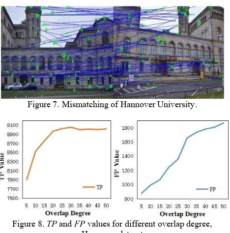
To further interpret the overlap result of the proposed method and compare it with VocMatch, the TP, FP, FN and TN values of our complete datasets were calculated. Again exhaustive matching served as ground truth. The results are showed in Tab. 3. The values in brackets are the differences to VocMatch; red means the VocMatch value is smaller than that of the proposed method, green means it is larger. A larger TP is calculated using our method, as well as the smaller FN and FP; we thus obtain a slightly better result than VocMatch does. This can also be concluded from Fig. 10 (see discussion below). In addition, Tab. 3 shows that we achieve a recall of about 50% (this means we find about half of the overlapping image pairs) and a precision of more than 85%, The FP value is not equal to zero, which means some image pairs are assumed to overlap by our algorithm, but they don’t actually do so. This frequently occurs due to mismatching. The two images shown in Fig. 7 depict the right and left side of the main building of Hannover University and do not overlap, however, the building is partly symmetric and thus there exist some conjugate points. Most of these false point pairs are detected during matching using the epipolar geometry constraint. Thus this is not a question we need to consider in our work.
Fig.8 shows the TP and FP values for Hannover University as a function of the overlap degree C. TP increases as C grows when C is smaller than 20, after that, it tends to be stable, on the other hand FP increases nearly linearly with C. Given a small C, the average degree of similarity S will be larger, such that some actually overlapping image pairs with small S value may be missed. As C increases, the average value of S will decrease, and image pairs with smaller S values are considered to be
overlapping at the risk that some incorrect image pairs (as Fig. 7 shows) are classified into the overlapping set. This result motivated us to select C=20 for our experiments.
Actual positive Actual negative Predicted positive 6.70 (-0.14) 1.18 (+0.09) Predicted negative 6.13 (+0.14) 158.43 (-0.09)
UAV + close range images
Actual positive Actual negative Predicted positive 8.97 (-0.10) 1.24 (+0.08) Predicted negative 9.376(+0.10) 81.44 (-0.08)
Hannover University
Actual positive Actual negative Predicted positive 29.86 (-2.38) 4.26 (+0.89) Predicted negative 31.25 (+2.38) 189.88 (-0.89)
Notre dame
Table 3. Derived Confusion Matrices (values in brackets indicate differences to VocMatch results)
Figure 7. Mismatching of Hannover University.
Figure 8. TP and FP values for different overlap degree, Hannover dataset
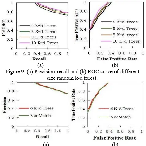
In Fig. 9, we show the precision-recall and ROC graphs of different sizes of random k-d forest. According to Fig. 9 (a) and (b), the 4 k-d trees give the worst overlap result, although not by a large margin. As the size of the random k-d forest increases, the overlap result becomes slightly better. The 6 k-d trees and the 8 k-d trees are almost at the same level. The result of 10 k-d trees is again a little better. By analysing Fig. 5, the computational time increases linearly as the size of the k-d random forest grows. Fig. 9 shows that the overlap result is only improved by a little margin. Considering the time efficiency and the overlap result, we choose 6 k-d trees as the best compromise for our experiments.
Fig. 10 shows the difference of the overlap evaluation between the proposed method (k =6) and VocMatch. From the precision-recall and ROC graphs, the overlap results of the proposed method and VocMatch are roughly the same as a whole, however, our approach is slightly better than VocMatch for a small false positive rate and a recall value lower than about 0.7. This means that, based on the experimental results presented here, if those two methods find the same number of green pixels (shown in Fig. 6(c)), the proposed method would find slightly less blue pixels than VocMatch.
(a) (b)
Figure 9. (a) Precision-recall and (b) ROC curve of different size random k-d forest.
(a) (b)
Figure 10. (a) Precision-recall and (b) ROC curve of different methods.
5. CONCLUSIONS
In this paper, a method based on a random k-d forest has been proposed to efficiently determine the mutual overlap of a large set of unordered images. The experimental results confirm that the proposed method performs rather well. To demonstrate the quality of the results we fed them into a sfm pipeline and visualised the outcome. To assess the time efficiency of our method we compared it to two other approaches. The results show that the proposed method is the most efficient one. For assessing our results numerically, we derived precision-recall and ROC curves. They confirm that the proposed method can obtain good overlap results.
Nevertheless, a number of open questions exist. Besides the relatively large number of false positive results (see Fig. 9(b)) we need further clarification about the sensitivity of the method with respect to a number of free parameters (the min. no. of points per image pair, the min. no. of images per cluster, the overlap degree etc). In terms of the methodology, a better selection for the splitting hyperplane in constructing the k-d trees is assumed to bring better results. We plan to investigate these questions in the near future.
ACKNOWLEDGEMENTS
The author Xin Wang would like to thank the China Scholarship Council (CSC) for financially supporting his PhD study at Leibniz Universität Hannover, Germany.
REFERENCES
Agarwal, S., Snavely, N., Simon, I., Seitz, S. M., and Szeliski, R., 2009. Building Rome in a day. ICCV, pp.72-79.
Arya, S., Mount, D. M., Netanyahu, N. S., Silverman, R. and Wu, A. Y., 1998. An optimal algorithm for approximate nearest neighbor searching in fixed dimensions. ACM, 45(6), pp. 891– 923.
Davis, J., Goadrish, M., 2006. The relationship between Precision-Recall and ROC Curves. Proc. 23rd Int. Conf. Machine Learning, pp: 233-240.
Farenzena, M., Fusiello, A., and Gherardi, R., 2009. Structure-and-motion pipeline on a hierarchical cluster tree. ICCV Workshop, pp. 1489-1496.
Frahm, J. M., Fitegeorgel, P., Gallup, D., Johnson, T., Raguram, R., and Wu, C., et al., 2010. Building Rome on a Cloudless Day. ECCV, 6314, pp.368-381.
Hartmann, W., Havlena, M., and Schindler, K., 2016. Recent developments in large-scale tie-point matching. ISPRS Journal of Photogrammetry & Remote Sensing, 115, pp.47-62.
Hartmann, W., Havlena, M., Schindler, K., 2014. Predicting Matchability. ICPR, pp.9-16
Havlena, M., Torii, A., Pajdla, T., 2010. Efficient structure from motion by graph optimization. ECCV, pp.100-113. Havlena, M., Schindler, K., 2014. VocMatch: Efficient Multiview Correspondence for Structure from Motion. ECCV, 46-60.
Havlena, M., Schindler, K. VocMatch. https://www1.ethz.ch/igp/photogrammetry/research/vocmatch. (accessed 01.12.2016).
Lowe, D.G., 2004. Distinctive Image Features from Scale-invariant Keypoints. IJCV, 60(2), 91–110.
Li, D.R., Yuan, X.X., 2012. Error processing and Reliability Theory. WuHan University Press, Wuhan, 229-233.
Mayer, H., 2003. Robust orientation, calibration, and disparity estimation of image triplets. DAGM, 281-288.
Mikulik, A., Perdoch, M., Chum, O., Matas, J., 2013. Learning vocabularies over a fine quantization. IJCV 103 (1), 163-175. Muja, M. Lowe, D.G., 2009. Fast approximate nearest neighbors with automatic algorithm configuration. VISAPP, 331–340.
Muja, M., Lowe, D.G., 2012. Fast Matching of Binary Features. Computer and Robot Vision, 404-410.
Muja, M., Lowe, D.G., 2014. Scalable nearest neighbor algorithms for high dimensional data. IEEE PAMI, 3(11), 2227-2240.
Nistér, D., Stewenius, H., 2006. Scalable Recognition with a Vocabulary Tree. ICPR, 2161-2168.
Robinson, J.T., 1984. K-D-tree splitting algorithm. IBM Technical Disclosure Bulletin, 27(5), 2974–2977.
Sarma, T.H., Viswanath, P., Reddy, B.E., 2013. Single pass kernel k-means clustering method. Sadhana-Acad. P. Eng. S., 38(6), 407–419.
Silpa-Anan, C., Hartley, R., 2008. Optimised KD-trees for fast image descriptor matching. CVPR, 1-8.
Sivic, J., Zisserman, A., 2003. Video Google. A Text Retrieval Approach to Object Matching in Videos. ICCV, 1470.
Snavely, N., Seitz, S. M., Szeliski, R., 2008a. Modeling the world from internet photo collections. IJCV, 80(2), 189-210. Snavely, N., Seitz, S. M., Szeliski, R., 2008b. Skeletal graphs for efficient structure from motion. CVPR, 1-8.
Snavely, N. Photo Tourism.
Sunil, A., 1998. An optimal algorithm for approximate nearest neighbor searching in fixed dimensions. Journal of the ACM, 45(6), 891–923.
Vedaldi, A., Fulkerson, B., 2008. VLFeat: an open and portable library of computer vision algorithms.
Wu, C., 2013. VisualSFM: Towards linear-time incremental structure from motion. 3DV, 127-134.
Wu, C. VisualSFM. http://ccwu.me/vsfm/ (accessed 10.12. 2016).