FAST AND RESISTANT PROCRUSTEAN BUNDLE ADJUSTMENT
Andrea Fusiello∗and Fabio Crosilla
DPIA - University of Udine Via Delle Scienze, 208 - 33100 Udine, Italy
e-mail: [email protected]
Commission III, WG III/1
KEY WORDS:Bundle adjustment, Orthogonal Procrustes, Block relaxation, Robust statistics
ABSTRACT:
In a recent paper (Fusiello and Crosilla, 2015) a Procrustean formulation of the bundle block adjustment has been presented, with a solution based on alternating least squares. This paper improves on it in two respects: it introduces a faster iterative scheme that minimizes the same cost function, thereby achieving the same accuracy, and makes the method resistant to rogue measures through iteratively reweighted least-squares. Empirical results confirm the effectiveness of these enhancements.
1. INTRODUCTION
Orthogonal Procrustes Analysis (OPA) is a very useful tool to perform the direct least squares solution of similarity transfor-mation problems in any dimensional space. At first, it was used for the multidimensional rotation and scaling of different matrix configuration pairs (Sch¨onemann, 1966, Sch¨onemann and Car-roll, 1970). Successively, the solution was generalized (GPA) for the simultaneous least squares matching of more than two corre-sponding matrices (Gower, 1975, Ten Berge, 1977). Anisotropic OPA is referred instead to the case where the class of transforma-tions is extended to anisotropic scaling of points or coordinates. For these problems (Gower and Dijksterhuis, 2004) suggest an iterative procedure where each variable is alternatively estimated while keeping the others fixed. This scheme is calledblock re-laxation(de Leeuw, 1994) oralternating least squares(Young et al., 1976). While an iterative solution with guaranteed conver-gence was described by (Bennani Dosse and Ten Berge, 2010) for the cases of pre- and post-scaling of the columns, no analogous property is known in the literature for rows scaling. Different versions of anisotropic GPA are described in (Lingoes and Borg, 1978), (Gower and Dijksterhuis, 2004), (Commandeur, 1991) and (Bennani Dosse et al., 2011) (they differ on where the scaling is applied).
In the field of terrestrial laser scanning GPA has been already applied to the registration of multiple 3-D models (Beinat and Crosilla, 2001, Toldo et al., 2010). In the field of photogramme-try, (Crosilla and Beinat, 2002) applied the GPA to the solution of block adjustment by independent models, while (Garro et al., 2012) applied OPA (with anisotropic row-scaling) to solve the ex-terior orientation problem. In a recent paper (Fusiello and Crosil-la, 2015) the Procrustean solution of the classical bundle block adjustment has been described. The method allows to obtain the same results of the classical least squares solution, without any linearization of the collinearity equations and without any a pri-ori information about the exterior pri-orientation parameters. The proposed method is based on the algorithms of the anisotropic Procrustean analysis and is implemented as a block relaxation procedure.
In this paper, an enhanced version of the above mentioned algo-rithm is presented. At first, a faster iterative solution of the same
∗Corresponding author
minimization problem is developed, that allows to obtain a reduc-tion of one order of magnitude w.r.t. the execureduc-tion time required by the original algorithm. This new relaxation scheme solves an anisotropic GPA with row-scaling using the same framework of the GPA solution (Gower, 1975). Furthermore, a robust objective function is introduced that makes the method resistant to outliers. The new scheme, based on Iteratively Reweighted Least Squares (IRLS), achieves reliable results also in the presence of a percent-age up to 10% of outliers.
2. PROBLEM FORMULATION
Let us now consider mimages depicting the same n 3-D tie-pointss1. . .sn. In thebundle block adjustmentproblem it is
required to simultaneously find the image exterior orientation pa-rameters and the tie-points 3-D coordinates that minimize a ge-ometric error, without introducing intermediate models, as op-posed to the block adjustment by independent models (Crosilla and Beinat, 2002). We review here the Procrustean solution to the free-network bundle block adjustment problem presented by (Fusiello and Crosilla, 2015).
We start from the collinearity equations for one camera:
pj=ζ−j1R(sj−c) (1)
where
sjis the coordinate vector of thej-th tie-point in the external
system;
cis the coordinate vector of the projection centre in the ex-ternal system;
ζj is a positive scalar proportional to the “depth” of the
point, i.e., its distance to the plane containing the projection centre and parallel to the image plane;
Ris the rotation matrix transforming from the external sys-tem to the camera syssys-tem;
pjis the coordinate vector of the projectedi-th tie-point in
the camera system, where the third component is equal to −f, the principal distance or focal length.
Expressing (1) with respect tosjand transposing yields:
s⊺
j=ζjp⊺jR+c
⊺
and stacking the equations fornpointss1. . .sn, the following
matrix formulation is obtained:
wherePis the matrix by rows of image tie-point coordinates de-fined in the camera system,Sis the matrix by rows of tie-point coordinates defined in the external system,Zis the (positive) di-agonal matrix containing the depth of each tie-point.
Thus, for each imagei= 1. . . mit is possible to write
S=ZiPiRi+1c⊺i. (5)
In this formula the image coordinatesPiare known, but all the
other quantities are unknown. They can be recovered by mini-mizing the following error function:
m
where each term of the sum represents the difference vector be-tween 3-D tie-points (S) and the corresponding 2D points (Pi)
back-projected according to their estimated depths (Zi) and
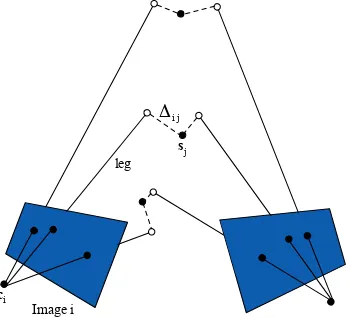
esti-mated image orientation (Ri,ci) of imagei. Let us call∆ijeach
individual difference vector relative to exposurei= 1. . . mand tie-pointj = 1. . . n(see Fig. 1). Overall, what is being min-imized is the length of the residuals∆ijfor each exposure and
each tie-point, in a least-squares sense.
s
Figure 1. The “legs” are line segments emanating from image points. The Procrustean bundle adjustment optimizes camera orientation and the length of each leg so as to bring the legs’ endpoints as close as possible to each other, i.e., minimizing the length of the∆ij.
Please note that ifZiwere known, the problem would reduce to
a GPA (see Appendix C), where the point sets to be aligned are theZiPi i= 1. . . m. On the other hand, computingZigiven
all the other variables is independent in each camera, and the so-lution, originally developed by (Garro et al., 2012), is reported in App. B. This observation underlies both the solutions of (Fusiello and Crosilla, 2015) and the novel one proposed in this paper.
3. PREVIOUS SOLUTION
In (Fusiello and Crosilla, 2015) a solution to (6) is proposed, it-erating between the following stages:
• assuming all theZi known, computeRi,ci by solving a
GPA problem (see App. C);
• set the putative 3-D pointsSto the centroids
S= 1
• solve forZiindependently in each image (see App. B):
Zi= (PiPi⊺⊙I)
−1
(PiRi(S⊺−ci1⊺)⊙I). (8)
The same formulation as (6) has been described at pg. 129 of (Commandeur, 1991), under the name STIMIDIO. The iterative solution proposed there is different from ours, though.
4. THE NEW SOLUTION: AGPA
The previous solution consists of two nested cycles, with a GPA as the inner one. This paper proposes a new iterative scheme without inner cycles, that has the same structure as the GPA, and therefore will prove to be faster.
Let us introduce theAnisotropic Generalized Procrustes Anal-ysis (AGPA), which extends GPA (described in App. C) with anisotropicrow-scaling for each individual model, and minimizes the following least squares objective function:
m
the same set ofnpoints inmdifferent coordinate systems.
LetP′
i =ZiPiRi+1c⊺i, by the same token as in the GPA
(Com-mandeur, 1991), the problem is equivalent to minimize
m
whereSis the centroid:
S= 1
This is the same objective function of (6), hence AGPA solves the bundle adjustment problem as formulated in Sec. 2.
Algorithm 1AGPA
Input: a set of 3-D modelsPi i= 1. . . m
Output: translationci, attitudeRiand scaleZiof each model
1. InitializeZi=IandPi′=Pi ∀i
2. Compute centroidS= 1
m
4. Iterate from step 2. until convergence of
m
The solution corresponds to a free adjustment, as it does not in-volve any object space constraint. In fact, the global scale of the solution is discretionary, and only the ratios of theZiare
rele-vant. Therefore, at each iteration theZiare normalized to unit
average, in order to avoid degeneracy. Moreover, negative values are clipped to zero in step (c).
Ground control points can be incorporated as in (Crosilla and Beinat, 2002).
As it will be shown in Sec. 6., this method has the same accuracy and convergence properties of the one reported by (Fusiello and Crosilla, 2015), but it is considerably faster.
5. RESISTANT AGPA
In real-world applications two issues must be considered, in order for any bundle adjustment method to be applicable. First, not all points are visible in all the images, so thePimatrices have some
unspecified entries.
Second, when tie-points have been obtained automatically – a very common trend (e.g. (Hartmann et al., 2015)) borrowed from the structure-from-motion literature – some of them are rogue points that would skew the Procrustean least square estimate, if proper countermeasures are not taken. This is particularly dan-gerous since the Procrustes procedure is fully automatic and does not require any a-priori information about the unknowns.
The first issue is handled as proposed in (Crosilla and Beinat, 2002), where for each matrixPi, a diagonal matrixMi can be
inserted, containing unit values along the main diagonal in case the corresponding row ofPiis specified and zero on the contrary.
As a result, the cost function is rewritten as:
m
where the centroidS, is now defined as:
S=
Resistance to outliers can be obtained, following (Verboon and Heiser, 1992), by substituting the least squares cost function of the classical Procrustes method with specific robust cost func-tions, and solving the resulting minimization problem with Iter-atively Reweighted Least Squares (IRLS) (Holland and Welsch, 1977).
This technique iteratively solves weighted least squares problems where the weights are estimated at each iteration by analysing the residuals of the current solution. The weights are assigned by a specificweight functionin such a way to penalize outliers and promote inliers.
In our case, the weighted cost function is:
m
whereW is a diagonal matrix containing the positive weights W(j, j)for each point.
The solution to the weighted version of the problem is the same as in AGPA, with the following substitutions:
Pi←QiPi S←QiS 1←Qi1 with Qi=MiW 1/2
.
Please note that the matrixW is not defined for each exposure, meaning that we conservatively attributeoutlyingnessto tie-points, as opposed to their image projections.
Several weight functions have been proposed in the literature; the ones offering greatest resistance to outliers are the so-called hard redescenders, that assign zero weight to points with resid-ual higher than a threshold. Among them we picked the popular bisquare (a.k.a. biweight) function (Mosteller and Tukey, 1977):
W(j, j) =
where the tuning constantkis chosen, as customary, so as to yield a reasonably high efficiency in the normal case, and still offers protection against outliers. In particular,k = 4.685σproduces 95-percent efficiency when the errors are normal with standard deviationσ. The latter is estimated robustly from the median ab-solute deviation (MAD) of the residuals asσ=M AD/0.6845.
In our case the residuals are defined as:
rj=
Algorithm 2RAGPA
Input: a set of 3-D modelsPi, Mi i= 1. . . m
Output: translationci, attitudeRiand scaleZiof each model
1. InitializeW =I and Zi=I, Pi′=Pi ∀i
2. Solve AGPA:
(a) Compute centroidS=
m
P
i=1
Mi
−1m
P
i=1
MiPi′
(b) Register each modelPitoS:
i. LetQi=MiW1/2andqi= diag-1(Qi)
ii. ComputeRi=Udiag(1,1,det(U V⊺))V⊺
withU DV⊺=P⊺
iQiZi(I−(qiq⊺i)/(q
⊺
iqi))QiS
iii. Computeci= (QiS−ZiQiPiRi)⊺qi/(q⊺iqi)
iv. ComputeZi=(PiPi⊺⊙I)− 1(P
iRi(S⊺−ci1⊺)⊙I)
v. UpdateP′
i =ZiPiRi+1c⊺i
vi. Compute residuals
rj= m
P
i=1
kS(j,:)−P′
i(j,:)k 2
2 j= 1. . . n
(c) Iterate from step (a) until convergence of residual
n
P
j=1
rj
3. Compute weightsW(j, j) = (|rj/k| ≤1)· 1−(rj/k)2 2
4. Iterate from step 2. until convergence of weights
It is worth noting that the computation of the centroidS does not involve the IRLS weightsW but onlyMi, and thatZidoes
not depend on the weights at all, as all computations, although in matrix form, are essentially point-wise, so any unspecified value in thej−throw ofPionly reflects to thej−thdiagonal value of
Zithat should be ignored. For the same reason it does not make
sense to down-weight outliers in the computation ofZi.
6. EXPERIMENTS
In this set of experiments, we tested (R)AGPA on repeated trials with simulated data. The aim was to assess i) its resistance to out-liers, ii) the increase in speed w.r.t. (Fusiello and Crosilla, 2015) and iii) the accuracy and failure rate. The comparison with pho-togrammetric bundle adjustment would have been pointless here because AGPA minimizes the same cost function as (Fusiello and Crosilla, 2015), which in turn has been already compared to pho-togrammetric bundle adjustment for accuracy.
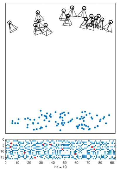
We followed the same validation protocol as in (Fusiello and Crosilla, 2015). For each trial,n3-D tie-points have been ran-domly generated in a sphere of unit radius1centred on the origin. Sixteen random cameras (m = 16) looking toward the origin have been positioned in a60◦sector of the sphere, at an average distance ofdunits from the origin. The focal length has been chosen so as to yield a view angle of{60◦,120◦}with an image size of1000×1000pixels. Random noise with unit variance has been added to the image coordinates. Missing points have been simulated by zeroing random elements in the visibility matrix. Outliers have been generated with uniform random coordinates in[−500,500]. A sample simulated scene is shown in Fig. 2.
The first experiment was designed for characterizing the failure rate, i.e., counting how many times our algorithm failed to reach the correct solution in 100 random trials, starting with the usual
1In these experiments on simulated data, measures are in arbitrary
“units”.
0 10 20 30 40 50 60 70 80 90
nz = 10 0
5
10
15
Figure 2. Top: A depiction of a simulated scene (cameras and points) used in the experiment (m= 16,n= 192, d= 10, p= 36); Bottom: the simulated visibility matrix, showing which point (x-axis) is visible in which image (y-axis). The outliers (10) are shown in red.
uninformed initialization (Z = 1). A random noise with 1 pixel standard deviation has been added to image coordinates. The pa-rameters considered in this simulation are the distancedof the camera from the origin and the numberpof tie-points visible in each image.
For each value ofd={2,10,20}3-D tie-points have been stre-tched in theXY plane so as to fit in the view frustum, while the Zrange is kept constant (to the original two units), so as to give rise to increasing values for the distance toZ-range ratio, namely {1,5,10}respectively.
The number of visible tie-points per image has been set top=
{18,36,54}. When the number of images and the number of vis-ible tie-points per image are fixed, total number of points and the ray multiplicity become dependent. In one case the total num-ber of points has been kept fixed ton = 96and the ray multi-plicity took the values{3,6,9}. In another case ray multiplicity has been fixed to 3 and the total number of points took values n={96,192,288}.
Figure 3 reports the results, that are aligned with those published in (Fusiello and Crosilla, 2015). The digest is that when the ray multiplicity is greater than 3 (top row,p={36,54}) the conver-gence rate is 100%. The case of ray multiplicity= 3is shown in the bottom row.
0
camera distance points per image
10 36
camera distance points per image
10 36
2 54
Figure 3. Failure rate of AGPA as a function of camera dis-tance d and number of tie-points visible in each image. Top row: Corresponding ray multiplicity values are[3,6,9], where n= 96. Bottom row: Corresponding total number of points are
[96,192,288], where the ray multiplicity is fixed to 3. Left/right column correspond to60◦/120◦field of view, respectively.
0
camera distance points per image
10 36
Figure 4. Median RMS error of AGPA as a function of cam-era distancedand number of tie-points visible in each imagep. The error is in percentage with reference to points distributed on a unit sphere. Top row: Corresponding ray multiplicity values are[3,6,9], wheren = 96. Bottom row: Corresponding total number of points are[96,192,288], where the ray multiplicity is fixed to 3. Left/right column correspond to60◦/120◦field of view, respectively.
In summary,AGPA has the same convergence rate and accu-racy than (Fusiello and Crosilla, 2015).
In the experiment aimed at assessing the resistance to outliers of RAGPA the parameters were set to: m = 16, n = 96, d = 10, p = 36. An increasing number of outliers has been added and 100 trials for each contamination level have been run. The results, reported in Fig. 5, indicates abreakdown point at 10%.
0 2 4 6 8 10 12 14 16 18
Figure 5.MeanandmedianRMS error vs percentage of outliers (m = 16, n = 96, d = 10, p = 36). The RMS error is in percentage with reference to points distributed on a unit sphere.
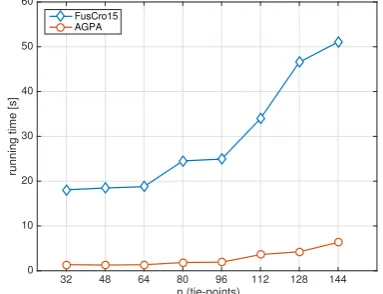
In the experiment aimed at assessing the speed-up of AGPA (MAT-LAB implementation) with respect to (Fusiello and Crosilla, 2015) (original MATLAB implementation by the authors) the parame-ters were set to: m = 16, d = 10and the ray multiplicity was set to 6. The number of pointsmhas been increased from 32 to 144, and the average running time over 20 independent trials has been recorded. The results are reported in Fig. 6, which shows thatAGPA is at least of one order of magnitude faster than (Fusiello and Crosilla, 2015).
32 48 64 80 96 112 128 144 d = 10, ray multiplicity =6) for(Fusiello and Crosilla, 2015)
andAGPA.
The tests on the same real datasets used in (Fusiello and Crosilla, 2015) confirm the outcome of the simulations. On the Herz-Jesu-P25 image-set (Strecha et al., 2008) the running time goes from 130s to 30s, whereas on the Hessigheim data (Cramer, 2013) it decreases from 460s to 100s at equal accuracy.
7. CONCLUSIONS
Crosilla, 2015). This new formulation solves the same minimiza-tion problem of its precursor but it isconsistently faster. As the previous version, the method achieves thesame accuracyof the classical photogrammetric bundle adjustment without any lin-earization of the collinearity equations and without any a priori information about the exterior orientation parameters. The robust cost function allows to tolerate up to 10% of outliers, by reducing their influence with a suitable weight function.
Future work will aim at characterizing the convergence of the method and possibly improving the breakdown point value.
REFERENCES
Beinat, A. and Crosilla, F., 2001. Generalized procrustes anal-ysis for size and shape 3d object reconstruction. In: Gruen and Kahmen (eds), Optical 3-D Measurement Techniques, Wichmann Verlag, pp. 345–353.
Bennani Dosse, M. and Ten Berge, J., 2010. Anisotropic orthog-onal procrustes analysis. Journal of Classification 27(1), pp. 111– 128.
Bennani Dosse, M., Kiers, H. A. L. and Ten Berge, J., 2011. Anisotropic generalized procrustes analysis. Computational Statistics & Data Analysis 55(5), pp. 1961–1968.
Commandeur, J. J. F., 1991. Matching configurations. DSWO Press, Leiden.
Cramer, M., 2013. The UAV@LGL BW project - a NMCA case study. In: Fritsch (ed.), Photogrammetric Week ’13, Wichmann, Berlin/Offenbach, pp. 165–179.
Crosilla, F. and Beinat, A., 2002. Use of generalised procrustes analysis for the photogrammetric block adjustment by indepen-dent models. ISPRS Journal of Photogrammetry and Remote Sensing 56(3), pp. 195–209.
de Leeuw, J., 1994. Block-relaxation algorithms in statistics. In: H. H. Bock, W. Lenski and M. M. Richter (eds), Information Sys-tems and Data Analysis, Springer-Verlag, pp. 308 – 325.
Fusiello, A. and Crosilla, F., 2015. Solving bundle block ad-justment by generalized anisotropic procrustes analysis. ISPRS Journal of Photogrammetry and Remote Sensing 102, pp. 209– 221.
Garro, V., Crosilla, F. and Fusiello, A., 2012. Solving the PnP problem with anisotropic orthogonal procrustes analysis. In: Sec-ond Joint 3DIM/3DPVT Conference: 3D Imaging, Modeling, Processing, Visualization and Transmission, pp. 262–269.
Gower, J., 1975. Generalized procrustes analysis. Psychometrika 40(1), pp. 33–51.
Gower, J. C. and Dijksterhuis, G. B., 2004. Procrustes prob-lems. Oxford Statistical Science Series, Vol. 30, Oxford Uni-versity Press, Oxford, UK.
Hartmann, W., Havlena, M. and Schindler, K., 2015. Recent de-velopments in large-scale tie-point matching. {ISPRS}Journal of Photogrammetry and Remote Sensing pp. –.
Holland, P. W. and Welsch, R. E., 1977. Robust regression using iteratively reweighted least-squares. Communications in Statis-tics - Theory and Methods 6(9), pp. 813–827.
Lingoes, J. and Borg, I., 1978. A direct approach to individual differences scaling using increasingly complex transformations. Psychometrika 43(4), pp. 491–519.
Mosteller, F. and Tukey, J. W., 1977. Data analysis and regres-sion: a second course in statistics. Addison-Wesley Series in Behavioral Science: Quantitative Methods.
Sch¨onemann, P. and Carroll, R., 1970. Fitting one matrix to an-other under choice of a central dilation and a rigid motion. Psy-chometrika 35(2), pp. 245–255.
Sch¨onemann, P., 1966. A generalized solution of the orthogonal procrustes problem. Psychometrika 31(1), pp. 1–10.
Strecha, C., Von Hansen, W., Van Gool, L., Fua, P. and Thoen-nessen, U., 2008. On benchmarking camera calibration and multi-view stereo for high resolution imagery. In: IEEE Con-ference on Computer Vision and Pattern Recognition, pp. 1–8.
Ten Berge, J., 1977. Orthogonal procrustes rotation for two or more matrices. Psychometrika 42(2), pp. 267–276.
Toldo, R., Beinat, A. and Crosilla, F., 2010. Global registration of multiple point clouds embedding the generalized procrustes analysis into an ICP framework. In: Proceedings of the 5th Inter-national Symposium on 3D Data Processing, Visualization and Transmission.
Verboon, P. and Heiser, W., 1992. Resistant orthogonal procrustes analysis. Journal of Classification 9(2), pp. 237–256.
Wahba, G., 1965. A Least Squares Estimate of Satellite Attitude. SIAM Review.
Young, F., Leeuw, J. and Takane, Y., 1976. Regression with qual-itative and quantqual-itative variables: An alternating least squares method with optimal scaling features. Psychometrika 41(4), pp. 505–529.
APPENDICES
A EXTENDED ORTHOGONAL PROCRUSTES ANALYSIS
The termsProcrustes Analysisis referred to a set of least squares mathematical methods used to compute transformations among corresponding points (ormodels) belonging to a generick -dimen-sional space, in order to achieve their maximum agreement (e.g. (Gower and Dijksterhuis, 2004)). In particular, theExtended Or-thogonal Procrustes Analysis(EOPA) allows to recover the least squaressimilaritytransformation between two models.
Let us consider two matrices A andB containing two sets of numerical data, e.g., the coordinates ofnpoints ofRkby rows. EOPA allows to directly estimate the unknown rotation matrixR, a translation vectorcand a global scale factorzthat solves:
minimize
z,c,R kB−zAR−1c
⊺k2 F
subject to R⊺R=RR⊺=I, det(R) = 1
(17)
Given the definition of the Frobenius norm, the cost function can be written equivalently as:
tr((B−zAR−1c⊺
)⊺
(B−zAR−1c⊺
)) (18)
The rotation is given by
R=Udiag(1,1,det(U V⊺))V⊺
(19)
whereUandV are determined from the SVD decomposition:
A⊺
(I−11⊺
/n)B=U DV⊺
. (20)
Thedet(U V⊺)normalization guarantees thatRis not only or-thogonal but has positive determinant (Wahba, 1965).
Thediag operator constructs a diagonal matrix from a vector, whereasdiag-1
returns a vector containing the diagonal elements of its matrix argument.
Then the scale factor can be determined with:
z= tr(R
⊺A⊺(I−11⊺/n)B)
tr(A⊺(I−11⊺/n)A) . (21)
And finally the translation writes:
c= (B−zAR)⊺1/n.
(22)
B ANISOTROPIC EOPA
The AEOPA is an instance of the classical EOPA (Sch¨onemann and Carroll, 1970), generalized by the fact that the isotropic scale factorzis substituted by an anisotropic scaling characterized by a diagonal matrixZof different scale factors:
minimize
According to (Gower and Dijksterhuis, 2004), this can be defined asanisotropicEOPA with row scaling.
To obtain the least squares solution one has to define a Lagrangian function and set to zero the partial derivatives with respect to the unknownsR,cand the diagonal matrixZ, as in the EOPA case (details in (Garro et al., 2012)). The results are:
R=Udiag(1,1,det(U V⊺
where⊙is the Hadamard (or element-wise) product.
The reader can notice that whereas in the solution of the EOPA problem one can recover firstR, that does not depend on the other unknowns, then the isotropic scale factorz, and finallyc, in the anisotropic case the unknowns are entangled in such a way that there is no direct solution available. (Gower and Dijksterhuis, 2004) suggest an iterative procedure where each variable is alter-natively estimated while keeping the others fixed. This scheme is calledblock relaxation(de Leeuw, 1994) oralternating least squares(Young et al., 1976).
C GENERALIZED PROCRUSTES ANALYSIS
Generalized Procrustes Analysis (GPA) is a well-known tech-nique that generalizes the classical EOPA (Sch¨onemann and Car-roll, 1970) to the alignment of more than two point sets (or mod-els), represented as matrices. It minimize the following least
squares objective function:
the same set ofnpoints inmdifferent coordinate systems. The degenerate solutionzi= 0∀imust be avoided by imposing some
constraint onzi.
The GPA objective function has an alternative formulation in terms of the centroid. LetP′
i =ziPiRi+1c⊺i, the following
equiva-lence holds (Commandeur, 1991):
m
whereSis the centroid,
S= 1
The left-hand term of Eq. (28) is a rewriting of Eq. 9, hence the right-hand term of Eq. (28) can be minimized instead.
IfS were known a direct solution of the transformation param-eters of each modelPi with respect to the centroidS could be
found by EOPA withA = Piand S = B. As suggested in
(Commandeur, 1991), the unknown centroid can be iteratively estimated, in a block relaxation fashion, giving raise to the GPA algorithm (Algorithm 3).
Algorithm 3GPA
Input: a set of 3-D modelsPi i= 1. . . m
Output: translationcand attitudeRof each model andz
1. InitializeP′
i =Pi ∀i
2. Compute centroidS= 1
m
4. Iterate from step 2 until convergence of
m