3D WEIGHT MATRICES IN MODELING REAL ESTATE PRICES
A. Mimis
Dept. of Economic & Regional Development, Panteion University, Greece, - [email protected]
KEY WORDS : Spatial Econometrics, 3D, Spatial Analysis, Weight M atrices
ABS TRACT:
Central role in spatial econometric models of real estate data has the definition of the weight matrix by which we capture the spatial dependence between the observations. The weight matrices presented in literature so far, treats space in a two dimensional manner leaving out the effect of the third dimension or in our case the difference in height where the property resides. To overcome this, we propose a new definition of the weight matrix including the third dimens ional effect by using the Hadamard produ ct. The results illustrated that the level effect can be absorbed into the new weight matrix.
1. INTRODUCTION
The weights matrix is an important part of spatial modelling and is defined as the formal expression of spatial dependence between observations (Anselin, 1988). The weight matrices are used in spatial autocorrelation and spatial regression. Examples of different weights matrix definitions exist in the literature and are based on spatial contiguity, inverse distance and k nearest neighbours among others (Cliff and Ord, 1981).
Despite the recent developments in the 3D city models (Biljecki et al., 2015), the spatial econometric models treat the space in a 2D manner, leaving the third dimension (height) incorporated, where needed, into covariates. Especially in the case of real estate data the level of the apartments has a clear and documented influence on the price of the property and is always present in the models with the form of dummies. Our approach tries to overcome this limitation by devising matrices that capture the weight of the 3D space.
This can be easily achieved by using distance weights based on the three coordinates. In our case this cannot be adopted and include the level of an apartment as the third dimension, since the space is not isotropic i.e. the z dimension (height) has a different influence from the position (x,y). To solve that, two different weight matrices can be calculated; one in the usual manner and a new one based on the level of each apartment and then combine these two, by using the Hadamard matricial product.
This approach is superior in that a) it captures the full 3D space in a weight matrix while at the same time b) eliminate totally the space effect from the independent variables and c) gives naturally defined models. In the next session, the methodology of evaluating the weight matrices in the particular case of real estate data will be described alongside a spatial error model, followed by the description of the dataset and the results.
2. METHODOLOGY
In order to explore the relation between house prices and their characteristics, one could start by using a linear regression model given by:
� = � + � (1)
where y(nx1) is the vector of observation of the dependent variable, X(nxk) is the matrix of covariates, β(kx1) is the vector of parameters and ε is the error term. The assumption of independent observations adopted in the above model is not always appropriate leading us to biased or inconsistent estimators.
This problem can be treated by applying spatial regression models, for example the spatial error model (SEM ) were the spatial dependence app ears in the error term, and is given by:
� = � + �
� = � � + � (2)
where λ is the autoregressive parameter, W(nxn) is the weight matrix, u(nx1) and Wu are the vector and the spatially lagged errors term respectively and ε is the vector of idiosyncratic errors.
A central role in the spatial regression models plays the weight matrix W, which captures the way one observation is related to the other observations in a typical 2D way . This matrix is usually defined exogenously based on contiguity, distance or k-nearest and has diagonal elements equal to zero.
This approach is extended to 3D space by dividing the weight matrix W(nxn) into two components, the matrices S and H of the same dimension. The first matrix S describes the connection of the observations in the (x,y) space and is calculated in the usual manner, while the second matrix H describes the relation of the observations in the z dimension.
So the elements hi,j of the matrix represent the different
impact due to height difference (or level in our case), between observations i and j. It is therefore defined by :
ℎ, =
{
, � � = � ,∀ ≠ , � � = � ,∀ =
|� − � |�, � � ≠ �
(3)
where , ≥ are fixed parameters.
The International Archives of the Photogrammetry, Remote Sensing and Spatial Information Sciences, Volume XLII-2/W2, 2016 11th 3D Geoinfo Conference, 20–21 October 2016, Athens, Greece
This contribution has been peer-reviewed.
Finally, we combine both S and H spatial matrices into a general 3D matrix W, by multiplying them, element by element
= �⨂� = �, ∙ ℎ , ⋱ �,�∙ ℎ ,�
��, ∙ ℎ�, ��, ∙ ℎ�,
where is the Hadamard product (Dube and Legros, 2009).
So, by using this novel approach, the elements of the weight matrix W are a fraction of the elements of the planar weight matrix S based on the level difference between the apartments. For example assume that two apartments i and j have a 2D distance smaller than a given threshold and that the one is on the 2nd and the other on the 3rd level. Then �,=1
and ℎ, = / ∙ � , resulting in a weight �, = / .
Similarly, one can use this approach to extend any other spatial model for example the spatial lag model (SAR) or more complex models such as the SAC model (Lesage and Pace, 2009).
3. DATA
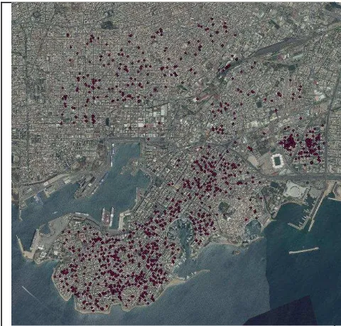
The study region is the municipality of Piraeus with an area of 11.2 square kilometers, where the biggest port of Greece is located. We have collected 1328 observations of asking prices for apartments for the period of September 2015 (M ap 1). Various apartment characteristics were collected and those used in the models are the price, the year of construction, the area in square meters, the level (floor), the geo-location (x,y coordinates) and the availability of parking, view, air condition, fireplace and awning. The later covariates were incorporated into the models as dummies with value of 1 if the amenity is present. The various attributes with their descriptive statistics are illustrated in Table 1.
Variable mean stdev
Price/square meter (€/m2) 1447.5 675.5
age (years) 20.8 17.5
area (m2) 79.6 27.9
parking (dummy) 0.49
view (dummy) 0.18
fireplace (dummy) 0.15 air condition (dummy) 0.26 awning (dummy) 0.23 level 0 (dummy) 0.11 level 1(dummy) 0.25 level 2 (dummy) 0.19 level 3 (dummy) 0.14 level 4 (dummy) 0.13 level 5 or more (dummy) 0.18
Table 1. Attributes of the apartments
M ap 1. Study area of Piraeus, Greece.
4. RES ULTS
In order to assess the presence of spatial dependence Moran’s I as well as the Lagrange M ultiplier (LM ) test (Anselin, 2005) have been used and the results are illustrated in Table 2.
Diagnostics Value1
Moran’s I (error) 76.3** Lagrange M ultiplier (lag) 100.3** Robust LM (lag) 82.9** Lagrange M ultiplier (error) 4607.5**
Robust LM (error) 4590.1**
Table 2. Diagnostics for spatial dependence
In Table 2, the z-value of Moran’s I (76.3) indicates that we can reject the null hypothesis of no spatial autocorrelation. Further, since both Lagrange M ultiplier statistics are significant (LM -lag and LM -error), we proceed to the robust version of the Lagrange M ultiplier. As both robust LM reject the null hypothesis of zero autoregressive parameter and the robust LM -error value is higher, we will adopt the spatial error model in our illustration.
So, an Ordinary Least Squares (OLS) model along with a SEM has been run into two flavours. In the first one, the level of the apartments has been included and the S matrix has been used while in the second case the levels has been excluded and the W matrix has been used.
For the data given, the S matrix is evaluated as a binary weights matrix based on a given distance cut -off of 700 metres. Then the H matrix has been set up by using equation (3) for a=0.1 and b=1.1. Finally the W matrix is defined by the Hadamard product. Both S an W has been row-normalized before used in the models.
1
** (*), statistically significant at 99% (95%) credible level. The International Archives of the Photogrammetry, Remote Sensing and Spatial Information Sciences, Volume XLII-2/W2, 2016
11th 3D Geoinfo Conference, 20–21 October 2016, Athens, Greece
This contribution has been peer-reviewed.
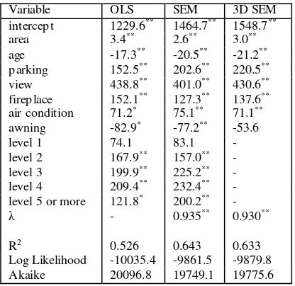
So in the regression model used, the price per square meter is the dependent variable whereas the rest of the variables described in Table 1 are used as covariates. The results of the models can be seen in Table 3.
Variable OLS SEM 3D SEM
intercept 1229.6** 1464.7** 1548.7**
area 3.4** 2.6** 3.0**
age -17.3** -20.5** -21.2** parking 152.5** 202.6** 220.5** view 438.8** 401.0** 430.6**
fireplace 152.1** 127.3** 137.6**
air condition 71.2* 75.1** 71.1** awning -82.9* -77.2** -53.6
level 1 74.1 83.1 -
level 2 167.9** 157.0** -
level 3 199.9** 225.2** - level 4 209.4** 232.4** - level 5 or more 121.8* 200.2** -
λ - 0.935** 0.930**
R2 0.526 0.643 0.633
Log Likelihood -10035.4 -9861.5 -9879.8 Akaike 20096.8 19749.1 19775.6
Table 3. Estimation results for the prices per square meters using OLS and SEM versions
From the results of all three models, we can see that the area, parking, view, fireplace, and air-condition variables have a significant positive impact on the price of the apartment. One the other hand, the age has a negative significant impact. Further the apartment levels, where included, increase the price of the property and further level 1 has a non-significant impact. Although all the findings are in good agreement with literature, the existence of awning has a negative impact on the price, not always significant, but still not expected.
As far as the marginal willingness-to-pay (M WTP) is concerned, in both the OLS and SEM models, the direct effect of a covariate is equal to the coefficient estimate of that covariate. So for example in the 3D SEM model (Table 3), the existence of a fireplace increases the price by 137 €/m2.
So comparing the M WTP between the two SEM models, we can see that in most of the cases, the covariates of the 3D SEM have a bigger impact on the price than the ones of the classic SEM .
The measures of fits used are the simple R2, the log-likelihood value (a higher value is associated with a better model) and the Akaike info criterion which is a function of log-likelihood adjusted for the number of covariates present (smallest value desired). The results for the two flavours of SEM indicate a better model fit in comparison with their OLS counterparts. The spatial error models provide similar results, despite the fact that when using W, the levels of the apartments are not included in the models, indicating that their effect has been completely absorbed by the weight matrix.
5. CONCLUS IONS
An effort has been made to include in the weight matrix, not only the flat two dimensional effect of the position but the third dimension i.e. height in the spatial econometric models. Our case study, illustrated promising results, where the different level effect of the apartments has been absorbed by the weight matrix.
In the future the effect/tuning of the parameters a, b must be examined.
REFERENCES
Anselin L., 1988. Spatial econometrics: Methods and models. Kluwer Academic Publishers, Dordrecht. .
Anselin L., 2005. Exploring Spatial Data with GeoDa: A Workbook. Spatial Analysis Laboratory (SAL). Department of Geography, University of Illinois, Urbana-Champaign, IL.
Biljecki F., Stoter J., Ledoux H., Zlatanova S., Coltekin A. (2015). Applications of 3D City Models: State of the Art Review. ISPRS International Journal of Geo-Information, Vol. 4, pp. 2842-2889.
Cliff A.D., Ord, J.K. 1981. Spatial processes: Models and applications. Pion, London.
Dube J., Legros D., 2009. A spatio-temporal measure of spatial dependence: An example using real estate data. Papers in Regional Science, Vol 92(1), pp. 19-30.
Lesage, J.P., Pace R.K., 2009. Introduction to spatial econometrics. CRC Press, Boca Raton.
The International Archives of the Photogrammetry, Remote Sensing and Spatial Information Sciences, Volume XLII-2/W2, 2016 11th 3D Geoinfo Conference, 20–21 October 2016, Athens, Greece
This contribution has been peer-reviewed.