A LABORATORY PROCEDURE FOR MEASURING AND GEOREFERENCING SOIL
COLOUR
´
A. Marqu´es-Mateua,∗, M. Balaguer-Puiga, H. Moreno-Ram´onb, S. Ib´a˜nez-Asensiob
a
Universitat Polit`ecnica de Val`encia (UPV), Department of Cartographic Engineering, Geodesy, and Photogrammetry, 46022 Val`encia, Spain – [email protected], [email protected]
b
Universitat Polit`ecnica de Val`encia (UPV), Department of Plant Production, 46022 Val`encia, Spain – [email protected], [email protected]
KEY WORDS:Soil, Colorimetry, CIE, GIS, Geomatics
ABSTRACT:
Remote sensing and geospatial applications very often require ground truth data to assess outcomes from spatial analyses or environ-mental models. Those data sets, however, may be difficult to collect in proper format or may even be unavailable. In the particular case of soil colour the collection of reliable ground data can be cumbersome due to measuring methods, colour communication issues, and other practical factors which lead to a lack of standard procedure for soil colour measurement and georeferencing. In this paper we present a laboratory procedure that provides colour coordinates of georeferenced soil samples which become useful in later processing stages of soil mapping and classification from digital images. The procedure requires a laboratory setup consisting of a light booth and a trichromatic colorimeter, together with a computer program that performs colour measurement, storage, and colour space transfor-mation tasks. Measurement tasks are automated by means of specific data logging routines which allow storing recorded colour data in a spatial format. A key feature of the system is the ability of transforming between physically-based colour spaces and the Munsell system which is still the standard in soil science. The working scheme pursues the automation of routine tasks whenever possible and the avoidance of input mistakes by means of a convenient layout of the user interface. The program can readily manage colour and coordinate data sets which eventually allow creating spatial data sets. All the tasks regarding data joining between colorimeter measure-ments and samples locations are executed by the software in the background, allowing users to concentrate on samples processing. As a result, we obtained a robust and fully functional computer-based procedure which has proven a very useful tool for sample classification or cataloging purposes as well as for integrating soil colour data with other remote sensed and spatial data sets.
1. INTRODUCTION
Vegetation maps are typical end products of remote sensing work-flows that have multiple potential uses in agricultural and envi-ronmental engineering as well as in soil science. Early authors on the subject of vegetation mapping from remote sensed images were already aware of the influence of soil spectral characteris-tics on the final maps due to the spectral mixing of signal coming from the vegetation response together with signals from the back-ground soil surface (Richardson and Wiegand, 1977, Tucker and Miller, 1977). The subject became a field of study on its own and its development led to the concept of ’soil line’ which is common nowadays (Baret et al., 1993, Gitelson et al., 2002).
There exist several methods to model the influence of soils in remote sensing applications. All those methods are somewhat based on underlying assumptions that may or may not be met in real applications. In particular soil lines derived entirely from the images are limited to points or areas located on bare soil pixels which is clearly a practical limitation.
It is also well accepted that soil type, together with roughness, water content and other factors, are soil parameters that can dis-tort the mathematical definition of soil lines. While roughness and water content parameters are highly variable in time and space, soil type is defined by a set of long-term characteristics that are routinely recorded in soil surveys. There are numerous applica-tions of survey data sets for quantitative analyses (Bouma, 1989) which include using those data in combination with remote sensed images and other spatially distributed datasets.
∗Corresponding author
Soil survey records include a number of physical, chemical, man-agement, and environmental characteristics such as soil colour. Colour is recorded with three attributes that can be related with the reflectance of soils in the visible region of the spectrum, and thus it has a clear relationship with remote sensed data as reported in previous research (Baumgardner et al., 1985).
There are two general approaches to computing soil and vegeta-tion fracvegeta-tions based either on visible and infrared data or on vis-ible data only (Gitelson et al., 2002). In any case, soil is not just a gray background and previous studies state that soil processing in remote sensing applications requires specific collection of soil spectral characteristics (Escadafal and Huete, 1992). Therefore, a procedure for collecting soil colour data in spatial format appears to be useful for methods based on data from the visible spectrum.
There is still another class of experimental studies where soil re-flectance data are used to find relationships between colour and soil properties. These studies include laboratory experiments (Tor-rent et al., 1983, Tor(Tor-rent and Barr´on, 1993), agricultural land-scape studies (S´anchez-Mara˜n´on et al., 1997, Gunal et al., 2008), and spatially based studies (Ib´a˜nez-Asensio et al., 2013, Moreno-Ram´on et al., 2014).
2. SOIL COLOUR
Standard texts on soil colour often begin stating that colour is the most obvious physical characteristic of soil (Simonson, 1993, Thwaites, 2006) which has practical applications in classifica-tion tasks (FAO, 2006, Soil Survey Staff, 2010), remote sens-ing (Baumgardner et al., 1985, Metternicht and Zinck, 2009), and mapping (Boettinger et al., 2010).
The physical and numerical framework for processing colour in-formation was established by theCommission Internationale de l’ ´Eclairage(CIE) in 1931 when a set of resolutions were pub-lished (Schanda, 2007). The CIE resolutions set the principles of modern colorimetry by gathering all the technical and scientific knowledge on colour of the time, and are still in use with some modifications. What follows is a brief summary of the resolutions from the soil laboratory standpoint.
Colour is conveniently represented in a three dimensional space such as the CIE RGB system. This is a physically-based sys-tem, and therefore is considered as a device independent system in contrast to digital devices that output RGB data in their par-ticular colour spaces. The CIE RGB system has obvious theo-retical interest, but it is not used in practice. Instead, a number of derivative spaces such as the CIE XYZ, CIE Yxy or CIELAB are preferred. There are closed formulas to convert colour data between those three colour spaces (CIE, 2004, Malacara, 2011).
The CIE 1931 XYZ colour space represents a colour stimulus with three numbers XYZ called tristimulus values, where Y rep-resents the luminance, that is, the total radiation reflected in the visible spectrum.
Tristimulus values can be converted to the so-called chromaticity coordinates using simple formulas:
x=X/(X+Y +Z); y=Y /(X+Y +Z) (1)
where x, y= chromaticity coordinates
X, Y, Z= tristimulus values
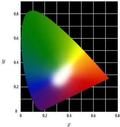
Chromaticity coordinates are normalised as a function of tris-timulus values that allows positioning colour stimuli in the Yxy colour space by means of the chromaticity diagram (Figure 1). The values ofxycarry the chromatic content of a colour stimu-lus, whereas the third dimension contains the achromatic compo-nent Y. Although chromaticity coordinates allow trained users to know a colour, they are not psychophysical correlates of human vision. There are, however, geometric formulas that give esti-mates of such correlates which are named dominant wavelength and excitation purity in the Yxy space (CIE, 2004).
The chromaticity diagram suffers from a lack of uniformity over its domain, which is a known issue when computing colour difer-ences with euclidean distances in the Yxy space. To overcome this problem, the CIE published a new color space called CIELAB in 1976 that is supossed to be quasi uniform. In the CIELAB space a colour is depicted with three coordinates namedL∗ (light-ness),a∗(red-green axis), andb∗(yellow-blue axis) in a solid based on the theory of opponent colours. L∗is a psychophysi-cal correlate of human perceived lightness. However,a∗andb∗ are not correlates of human perceived hue and saturation, but the CIELAB space provides formulas to calculate estimates of hue (hab) and chroma (C∗
ab) (CIE, 2004). TheL∗C∗hspace is
there-fore a psychophysical counterpart of the CIELAB space.
Figure 1: CIE chromaticity diagram
The CIELAB coordinates are computed as follows (CIE, 2004):
L∗ = 116
·(Y /Yn)1/3
a∗ = 500
·(X/Xn)1/3−(Y /Yn)1/3 (2)
b∗ = 200
·(Y /Yn)1/3−(Z/Zn)1/3
where L∗a∗b∗= CIELAB coordinates
X, Y, Z= tristimulus values of the observed sample
Xn, Yn, Zn= tristimulus values of reference white
The CIELAB space also provides formulas to compute colour differences. Given two colours (L∗
1, a∗1, b∗1) and (L∗2, a∗2, b∗2) the difference is (CIE, 2004):
∆E∗
ab= p
(L∗ 2−L∗1)
2+ (a∗ 2−a∗1)
2+ (b∗ 2−b∗1)
2 (3)
All the previous colour spaces were originally defined by means of visual experiments with human observers. The implementa-tion of those physically-based colour spaces in modern instru-ments are done with a spectrophotometric approach that calcu-lates tristimulus values with the sum of the product of three func-tions across the visible range of the electromagnetic spectrum. The expressions are (CIE, 2004):
X =
Z
λ
ρλ·Eλ·xλ dλ
Y =
Z
λ
ρλ·Eλ·yλ dλ (4)
Z =
Z
λ
ρλ·Eλ·zλ dλ
where ρλ= reflectance function of the specimen
Eλ= light spectral function
The spectrophotometric formulas take into account the three el-ements of colour, that is, the object that reflects light energy, the light source characteristics, and the observer (or sensor that de-tects the light). The colour matching functions represent a human observer with normal colour vision. These functions are pub-lished by the CIE (CIE, 2004) and must be somehow embedded in modern instrumentation. It is worth noting that in engineering applications the integrals in Equation (4) are replaced with sums.
Although CIE colour spaces define a rigorous framework to pro-cess colour data, the study of colour in soil science followed a different path. The first references to color in soil surveys date back to the last decade of the 19th century. The approach to com-municating colour in soil science was a visual procedure that al-lowed field surveyors to match the colours of soil samples with a collection of colour chips arranged in the so-called colour books (Figure 2). Although precursors of the CIE spaces already ex-isted at that time, the technological development of instruments together with the limited computing power made the CIE spaces unsuitable for practical uses. In 1941, the United States Depart-ment of Agriculture (USDA) published the first soil colour charts (Simonson, 1993) in a format which has remained to the present day (Munsell Color, 2000).
Figure 2: Visual assessment of soil colours with Munsell charts
The USDA published the colour charts in collaboration with the Munsell Color Company where a team of arstists and scientists leaded by A.F. Munsell developed a physical implementation of a colour solid. The colour solid was supposed to represent the whole domain of colours that were physically realizable with the colour technology available.
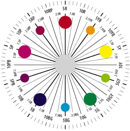
In the Munsell system, colours are arranged following an order in the three colour components: hue, value and chroma. It is there-fore a colour order system that is specially suited to making fast visual comparisons with suitable training. In the Munsell system the term ’value’ is used to denote an equivalent to luminance or lightness in the CIE spaces. There are clear similarities between the Munsell order system and the CIE spaces. For instance, the Munsell hue circle is very similar to the CIE chromaticity dia-gram. Note however that hues are arranged in opposite order in both representations (Figures 1 and 3).
Colour communication with Munsell charts is done with descrip-tions called Munsell notadescrip-tions. Notadescrip-tions are alphanumeric codes that describe a colour stimulus in terms of hue, value and chroma exactly in this order. Hue contains numbers and letters (R=red, Y=Yellow, B=Blue, and so on). Value and chroma are numbers. Each notation has an associated colour name. As an example a
notation 10YR6/4 has a colour name ’light yellowish brown. The three components are hue (10YR), value (6) and chroma (4).
Figure 3: Munsell hue circle
The use of CIE spaces is well suited to laboratory work since they allow high degree of automation and efficient processing of soil colour data. However, the laboratory setup must be estab-lished very carefully to reach maximum accuracy in the measure-ments (Torrent and Barr´on, 1993). The Munsell system, on the other hand, is still common use in soil science as observed in standard manuals (Soil Survey Division Staff, 1993). The coex-istence of two colour systems poses a problem of transformation between two different spaces. This problem is not yet solved with analytic formulas (Malacara, 2011) although there are a number of different approximate methods in the literature. We face this problem in Section 3.4 with a simple machine learning technique.
3. PROCEDURE OUTLINE
The requirements considered when designing the procedure were twofold. First, we sought a procedure such as not to interfere with standard soil analyses. Secondly, we needed to create ready to use datasets in spatial format.
The first requirement was met by allocating a specific room in the Soils Laboratory of the Universitat Polit`ecnica de Val`encia (UPV) as a dedicated colour laboratory. With this infrastructure, a small fraction of every soil sample can be processed to collect colour data in parallel with regular soil analyses.
The second requirement demanded a configurable computer envi-ronment in order to automate the measurement process as much as possible, and eventually to create the spatial databases. Af-ter assessing several options, we decided to write a program that fitted to our specific needs from the beginning.
Both criteria were taken into account when setting the processing routines of the procedure as outlined in Figure 4. The flowchart separates tasks done in the colour laboratory from those carried out in the soils laboratory.
Figure 4: Flowchart of the procedure
space used in this step depends on instrumentation characteris-tics. In our setup we used a trichromatic colorimeter that outputs coordinates in the CIE Yxy space. The coordinates are automat-ically converted to CIELAB coordinates provided that white ref-erence readings are available in the data set.
In the second step, CIE coordinates are transformed to Mun-sell notations using records contained in the training data set file which is labeled as ’TDS’ in Figure 4. For a description of the Munsell transformation see Section 3.4. This step is optional and depends on the existence or availability of the training data set.
Finally, the third step creates spatial data files on disk. This oper-ation requires a coordinate database (’CDB’ in Figure 4) contain-ing spatial coordinates of the sample points. It is the responsibil-ity of the user to create and maintain that database. The reference system of the coordinates must be consistent since the computer program that reads the file makes no assumption on this matter. This step requires the coordinate database to work properly. If, for any reason, the coordinate database is not available, the ouput will be a simple data table without spatial information. The final spatial database is labeled ’SDB’ in Figure 4.
3.1 Laboratory setup
The laboratory setup is a critical point to achieve maximum accu-racy and efficiency in soil colour processing (Torrent and Barr´on, 1993). The components of our setup are: colorimeter, light booth, datalogger, and uninterruptible power supply (UPS).
We used a non-contact trichromatic colorimeter that fits well to measuring granular specimens. The instrument was the Chroma Meter CS-100A by Konica Minolta (Konica Minolta, 1992). This class of instruments require careful mounting to keep the distance to the specimen constant. If that distance were not constant lumi-nance readings could not be compared among samples.
Another critical point is the geometry of illumination. We used a configuration known as 45◦/0◦geometry where light reaches the sample being observed at 45◦measured from the normal to the sample surface. That geometry avoids specular reflection, glare, and other unwanted optical effects, and ensures that recorded colours belong to soil samples rather than to light. The colour
Figure 5: Laboratory setup
sensor is mounted at 0◦from the normal to sample plane as seen in Figure 5.
We followed recommendations given by the instrument maker and by the CIE. Besides geometry, the recommendations also in-cluded the white plate and the illuminant used in the measurement process. We chose the CS-A20 white calibration plate which is part of the complementary equipment of the CS-100A colorime-ter (Konica Minolta, 1992). Regarding illuminant, we used D65 (Daylight 6500K) simulators as proposed by the CIE for colour experiments (CIE, 2004).
The setup is completed with the datalogger which takes care of communicating with the colorimeter by sending messages to the instrument and collecting back colour data. In our setup the dat-alogger was a regular PC computer running a computer program (Section 3.2) that also performed other tasks such as computing average values from raw measurements, reading auxiliary files and writing the final spatial databases.
The communication is done over a RS-232 serial line which was available in the computer. We used a special RS-232 cable called LS-A12 which has two connectors. One connector is the well-known DB9 which has 9 pins and was the most common con-nector until the advent of USB ports. The other concon-nector is a non-standard one called RP17-13RA-12SD created by Konica Minolta to fit the serial port located in the colorimeter frame.
It is important to note here that a time period of 30 minutes should be established before proceeding to measuring tasks. This pe-riod allows the light sources to reach their operating temperature which is necessary to avoid measurements deviations due to vari-ations in ambient light. The UPS contributes to maintain such uniform light conditions avoiding voltage variations.
3.2 Computer program
The computer program described in this section was codenamed CS-100A and is one major element of the procedure to measure and georeference soil samples. We developed this program with laboratory user’s needs in mind, and imposed ourselves several requirements such as multiplatform support, seamless integration in laboratory workflow, and connectivity with the colorimeter.
and is always available in standard installations. The module py-serial provides an interface to communicate with py-serial devices. This module is not part of the standard Python and must be in-stalled prior to running the application.
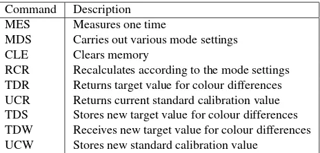
It should be stressed here that proper communication with the colorimeter was possible because the communication protocol was available (Konica Minolta, 2000). The documentation was very precise and allowed us to write the communication functions without problems. The protocol is asynchronous, so that first the program sends a message to the colorimeter, then the colorimeter does something and sends some data back to the program. The program should finally interpret and decode the received data in a convenient way. The three important aspects of the protocol are the communication parameters, the list of valid commands and the format of the received data.
The CS-100A instrument has a fixed configuration with the fol-lowing parameters:
• Baud rate: 4800
• Parity: even
• Data length: 7 bits
• Stop bits: 2 bits
The complete list of commands is shown in Table 1 although the most important for the program is ’MES’ which measures one time. The commands sent over the serial line have two fields, the command name and the delimiter that marks the end of the message. In this protocol the delimiter is a two character string with CR (carriage return) and LF (line feed). Therefore, in order to take a measure the program must send the message:
MES + <CR> + <LF>
The data sent back by the instrument consist of text strings with fields separated by commas. A typical string returned after send-ing a ’MES’ command looks like the followsend-ing:
"MES: OK00, 121.5, .3325, .3565"
The string contains the command name and the message that car-ries the measurement. The measurement has four fields. The first field (OK00) is an error code that in this particular string means that there were no errors. The three remaining areY xy coor-dinates. The second field (121.5) is the luminance in units of
cd/m2
. The units of luminance variable can be changed with a switch located in the battery chamber of the instrument. The third (.3325) and fourth (.3565) fields are chromaticity coordinatesx
andyrespectively.
Command Description MES Measures one time
MDS Carries out various mode settings
CLE Clears memory
RCR Recalculates according to the mode settings TDR Returns target value for colour differences UCR Returns current standard calibration value TDS Stores new target value for colour differences TDW Receives new target value for colour differences UCW Stores new standard calibration value
Table 1: Commands of CS-100A protocol
The first task performed by the program is to check the operat-ing system it is runnoperat-ing on. This is a simple but important step to guarantee multi-platform support. We successfully tested the program on Linux, Mac OS and Windows with exactly the same source code.
Next, the program reads a configuration file containing several variables. Those variables specify several disk locations to store data files, and other parameters such as the output spatial format or the serial port that provides colour data from the colorimeter. If the configuration file does not exist, then a default configuration is set by the program. After reading the configuration file into memory, the main graphical user interface is displayed on the screen (Figure 6).
Figure 6: Main window of the program
Figure 7: Configuration window
Before proceeding with the measurement tasks, users can change the configuration of the working environment. Configurable items include: output data files, auxiliary files, spatial format, and serial port (Figure 7). There are two output files to store measurements and a log of the session. The measurements file contains a table ofY xy coordinates in comma separated values (CSV) format. This file is suitable to be processed in other computing environ-ments. The log file contain more information such as timestamps and raw text strings recovered from the colorimeter.
The auxiliary files are the coordinates and the Munsell files. The former contains spatial coordinates of the samples to be processed, whereas the latter contains CIE coordinates of Munsell chips. Both files must be provided by the user and are optional in some sense, that is, if they are not available, the program can still run and generate meaningful outputs, but they are required to obtain full functionality. For instance, if the coordinates file is not avail-able the output will not be in spatial format.
format is probably the most common format in the fields of ge-ographic information systems (GIS) and geomatics. It was in-troduced by a commercial company and has become ade facto standard probably because the specification of the format is pub-licly available (ESRI, 1998). The geography markup languaje (GML) format, on the contrary, is a standard proposed by the Open Geospatial Consortium (OGC) and is ”an XML grammar for expressing geographical features” whose specification is avail-able in several official documents (OGC, 2010). Finally, the Geo-JSON is the most recent format of the three. GeoGeo-JSON is based on the JavaScript object notation (JSON) and is defined as ”a for-mat for encoding a variety of geographic data structures.” This format can be a valid option to send geographic data over com-puter networks or in mobile devices and use the concept of dic-tionary or associative array to pack the data (Sriparasa, 2013).
The last configurable item is the serial port that will be the entry point of colorimetric data. The names of such ports are platform dependent and is one of the points that our program manages at start time to show correct port labels regardless of the platform.
3.3 Program operation
As described in the previous section, the GUI is very simple and consists of two windows that allow measuring and configuring tasks. The main window has two sections as seen in Figure 6. The left half of the window has three text boxes and the right half contain a number of buttons with specific functions. A brief outline of the program operation and some recommendations are given below.
The first action of the user is to type the Sample ID in the entry located in the upper left section. The ID allows joining colour measurements with spatial coordinates and other data, therefore it must be unique. There are two special IDs (’w’ and ’white’) reserved to indicate measurements on the white calibration plate. It is common to start a measuring session with a reading on the reference white plate.
Below the sample ID entry there are two text boxes where colour measurements are shown as they are read from the colorimeter. The upper (and bigger) box contains all the measurements done on the current sample, whereas the bottom box contains mean values of the coordinates measured up to that point. The mean values of luminanceY and chromaticity coordinatesxyare up-dated after every new measurement.
In the right section there is a group of six buttons that allow ac-tions such as measuring colour coordinates, clearing the data to start a new measurement series, saving measured data, configur-ing the workconfigur-ing environment, exportconfigur-ing the data to spatial format, and stopping the program.
The ’Measure’ button sends a ’MES’ command to the colorime-ter to request a new measurement. Afcolorime-ter receiving the command, the instrument takes a new measurement and sends it back to the other side of the serial link. In the meantime, the program stays listening for any incoming data. When the new coordinates arrive, they are displayed on the measurement text box and the mean values are updated.
The natural way of measuring the colour of a sample is by read-ing a series of values. The program allows this and shows all the individual measurements and the mean values for each colour co-ordinate coco-ordinate (Y,xandy). If for any reason it is necessary to reject any previous measures, the user should click on button ’Clear’. This button removes any contents both in the text boxes and in memory, and awaits for a new measurement series.
If the data are correct the user should click on button ’Save’ to store the data on disk files. This button also removes any previous content from the text boxes and awaits for a new series. The mean values are stored in the file specified in the configuration window under the item ’Measurement’ of the ’Output files’ area. The individual raw measurements are recorded in the log file with timestamps just in case the user needs to check the whole session.
The ’Config’ button shows the configuration window (Figure 7) where the user can customise the environment. As described in the previous section, there are four configurable items: output files, auxiliary files, spatial format, and serial port.
Once the whole laboratory session has finished, the user should click on ’Export’ to create a spatial database containing colour in-formation about the processed samples. When clicking this but-ton, several actions take place in the background in a transparent fashion for the user. First, the program searches for the spatial coordinates database. If this file does not exist, it will not be pos-sible to create the spatial database. In this event, the program will print a warning message. Next, the program searches for the Munsell file with the CIE coordinates of the Munsell colour chips to transform CIE coordinates into Munsell notations. If both files exist, the the user ends up with a spatial database containing point geometries and an attribute table with CIE coordinates as well as with Munsell notations. It should be noted that the program also calculates CIELAB coordinates and writes them to the attribute table if white reference readings are found in the data file.
It is convenient to highlight a couple of key points before closing this section. As stated above, there are several CIE colour spaces used in soil science, the Yxy and CIELAB spaces being the most commonly used in practice. It is worth noting that program CS-100A does not check the colour space of the Munsell data. It is the responsibility of the user to ensure that both, samples coor-dinates and Munsell chips coorcoor-dinates, are expressed in the same colour space. Otherwise, the results will contain errors. Likewise, it is necessary to measure soil samples under the same environ-mental light conditions of the Munsell charts measurements to obtain consistent results.
3.4 CIE to Munsell transformation
As mentioned above, one point of interest in soil colorimetry is to report colours as Munsell notations to ensure compatibility with common practice. While there are closed formulas to convert between CIE XYZ, CIE Yxy, and CIELAB spaces (CIE, 2004), in the case of transforming from CIE coordinates into Munsell notations such formulas do not exist. Instead, a number of ap-proximate methods can be found in the colorimetry literature. We addressed this problem with a non-conventional approach in soil colorimetry based on the k nearest neighbours (k-NN) tech-nique (Steinbach and Tan, 2009).
The goal of the k-NN method is to assign class labels to unknown objects. Those objects are just points in a multidimensional co-ordinate system. In our particular case, the obvious choice is to define the coordinate system with the three colour dimensions,
Y xyin the CIE Yxy space orL∗a∗b∗in the CIELAB space.
There are two datasets named test and training sets. The test dataset contains records that represent unknown objects, that is, objects whose classes are to be defined. The training dataset, on the contrary, contains objects with known classes that have been somehow assigned. Each record in both datasets holds the coor-dinates of a single object.
Then, the k nearest neighbours are selected and their labels re-tained. The label to be assigned to the test is chosen using a voting strategy, that is, the label with more votes or occurrences among the k neighbours will be selected.
The key points to be defined in the k-NN method are therefore (Steinbach and Tan, 2009):
• The set of labeled or known objects
• A distance or similarity metric
• The value ofk
• The method used to determine the class of the test objects
It is necessary to adapt those key elements to the problem of con-verting from CIE coordinates to Munsell notations. The set of labeled objects must be obviously the Munsell chips, that have to be observed with the colorimeter using the laboratory setup de-scribed above. The point here is that our labels are Munsell nota-tions, so that classifying test objects is analogous to set Munsell notations.
The metric used is the euclidean distance in the CIE space. In this respect, it is better to use CIELAB coordinates rather than
Y xy coordinates for colour uniformity reasons. The program described here will always use CIELAB coordinates if there are white calibration readings available.
The value ofkis one in our case since each class, that is each Munsell notation, contains only one member that corresponds to a particular colour chip. The method to determine the class of test objects makes no sense with a value ofk=1.
In summary, it is possible to convert CIE coordinates to Munsell notations using the k-NN method with a valuek =1. This is equivalent to select the notation of the nearest Munsell chip to the test sample. In spite of the simplicity of this method, there are several drawbacks that can be limiting in certain circumstances and have been studied in the literature (Steinbach and Tan, 2009).
Although the k-NN classification method can be easily imple-mented, we used theKNeighborsClassifier class from the Scikit-learn module (Pedregosa et al., 2011). This classifier pro-vides an interface to execute the k-NN method in a few lines of code.
The process requires importing the package:
>>> from sklearn import neighbors
The k-NN classification is a three-step process. First, a classifier object must be created specifying the number of neighbours that must be one in our problem:
>>> knn = neighbors.KNeighborsClassifier(1)
In the previous line it is possible to pass optional parameters to indicate the weighting scheme withweights=’uniform’or the metric withmetric=’euclidean’.
The second step requires two lists that contain the training dataset records (training) and the class labels (labels). The two lists are joined with thefitmethod:
>>> knn.fit(training, labels)
Finally, the classification of new data points is done withpredict:
>>> test class = knn.predict(test)
wheretestis a list that contains test records andtest classis an array of labels that allow classifiying the unknown records.
The parameters of the previous methods can be lists or arrays that should match in their dimensions. For instance,training
has dimensions m×n, where m is the number of training records and n is the number of dimensions of the space. The number of items in listlabelsmust be m and the dimensions oftestmust be u×n, where u is the number of test records and n the number of coordinates or dimensions of those test records.
3.5 Measurement routine
After setting up the laboratory and assembling all the compo-nents (light booth, colorimeter, computer, and so on) we defined a measurement routine based on user’s experience. The goals of the routine are to speed up the laboratory work sessions and to minimise errors.
The routine consists of the following steps:
1. Fill up a Petri plate with soil
2. Shake the plate to obtain a ’flat’ and ’homogeneous’ surface
3. Put the plate into the light booth
4. Measure colour coordinates
5. Take the plate from the booth and mix soil material
6. Repeat steps 2, 3 and 4
7. Repeat step 5
8. Repeat steps 2, 3 and 4
9. Save measurements to disk file
This routine provides three measurements per sample which al-lows being aware of possible deviations across measurements. It should be noted that small deviations are possible due to the granular nature of soil samples. It is for this reason that samples should be shaken before repeating a measure. When the user ac-cepts the measured values, the average is calculated and reported in the final data files.
The measurement routine can be complemented with reference white readings that should be inserted at regular intervals during the laboratory work session. These measurements are mandatory if CIELAB coordinates are needed.
4. CONCLUSIONS
The procedure described herein is an effective tool for users in-terested in studying soil colour in combination with other envi-ronmental and agricultural variables.
The idea of developing a tailored application allowed fitting the procedure to specific laboratory requirements and integrating co-lour processing in the laboratory workflow.
approach emulated reasonably well the visual matching process experienced by human observers that consists of assessing the minimum chromatic distance between a sample and a collection of colour chips.
In summary, the procedure presented in this paper covers all needs for soil colorimetry and creates spatial databases that can be used in environmental, agricultural and remote sensing applications.
REFERENCES
Baret, F., Jaquemoud, S. and Hanocq, J., 1993. About the Soil Line Concept in Remote Sensing. Advanced Space Research 13(5), pp. 281–284.
Baumgardner, M., Silva, L., Biehl, L. and Stoner, E., 1985. Re-flectance properties of soils. In: N. Brady (ed.), Advances in Agronomy, Vol. 38, pp. 2–44.
Boettinger, J., Howell, D., Moore, A., Hartemink, A. and Kienast-Brown, S. (eds), 2010. Digital Soil Mapping. Bridging Research, Environmental Application, and Operation. Springer.
Bouma, J., 1989. Using Soil Survey Data for Quantitative Land Evaluation. In: B. Stwart (ed.), Advances in Soil Science, Vol. 9, Springer-Verlag, pp. 177–213.
CIE, 2004. Colorimetry. Commission Internationale de l’ ´Eclairage.
Escadafal, R. and Huete, A., 1992. Soil optical properties and environmental applications of remote sensing. Interna-tional Archives of Photogrammetry and Remote Sensing 29(B7), pp. 709–715.
ESRI, 1998. ESRI Shapefile Technical Description. Environmen-tal Systems Research Institute.
FAO, 2006. World reference base for soil resources 2006. World Soil Resources Reports No. 103. Food and Agriculture Organi-zation of the United Nations.
Gitelson, A., Stark, R., Grits, U., Rundquist, D., Kaufman, Y. and Derry, D., 2002. Vegetation and soil lines in visible spectral space: a concept and technique for remote estimation of vege-tation index. International Journal of Remote Sensing 23(13), pp. 2537–2562.
Gunal, H., Ersahin, B., Yetgin, B. and Kutlu, T., 2008. Use of chromameter-measured color parameters in estimating color-related soil variables. Communications in Soil Science and Plant Analysis 39, pp. 726–740.
Ib´a˜nez-Asensio, S., Marqu´es-Mateu, A., Moreno-Ram´on, H. and Balasch, S., 2013. Statistical relationships between soil colour and soil attributes in semiarid areas. Biosystems Engineering 116(2), pp. 120–129.
Konica Minolta, 1992. Chroma Meter CS-100A. Instruction Manual. Konica Minolta.
Konica Minolta, 2000. Chroma Meter CS-100A. Communication Manual. Konica Minolta.
Malacara, D., 2011. Color Vision and Colorimetry: Theory and Applications. 2nd edn, SPIE Press.
Metternicht, G. and Zinck, J. (eds), 2009. Remote Sensing of Soil Salinization. Impact on Land Management. CRC Press.
Moreno-Ram´on, H., Marqu´es-Mateu, A. and Ib´a˜nez-Asensio, S., 2014. Significance of soil lightness versus physicochemical soil properties in semiarid areas. Arid Land Research and Manage-ment 28, pp. 371–382.
Munsell Color, 2000. Munsell Soil Color Charts. GretagMac-beth.
OGC, 2010. OpenGIS Implementation for Geographic Informa-tion - Simple feature access - Part 1. Open Geospatial Consor-tium.
Pedregosa, F., Varoquaux, G., Gramfort, A., Michel, V., Thirion, B., Grisel, O., Blondel, M., Prettenhofer, P., Weiss, R., Dubourg, V., Vanderplas, J., Passos, A., Cournapeau, D., Brucher, M., Per-rot, M. and Duchesnay, E., 2011. Scikit-learn: Machine Learning in Python. Journal of Machine Learning Research (12), pp. 2825– 2830.
Richardson, A. and Wiegand, C., 1977. Distinguishing Vegeta-tion from Soil Background InformaVegeta-tion. Photogrammetric Engi-neering and Remote Sensing 43(12), pp. 1541–1552.
S´anchez-Mara˜n´on, M., Delgado, G., Melgosa, M., Hita, E. and Delgado, R., 1997. CIELAB color parameters and their rela-tionships to soil characteristics in Mediterranean red soils. Soil Science 162(11), pp. 833–842.
Schanda, J. (ed.), 2007. Colorimetry. Understanding the CIE sys-tem. John Wiley & Sons.
Simonson, R., 1993. Soil color standards and terms for field use -history of their development. In: J.M. Bigham and E.J. Ciolkosc (ed.), Soil color, Soil Science Society of America, pp. 21–34.
Soil Survey Division Staff, 1993. Soil Survey Manual. USDA Handbook 18. Soil Conservation Service. U.S. Department of Agriculture.
Soil Survey Staff, 2010. Keys to Soil Taxonomy. 11th edn, USDA-Natural Resources Conservation Service.
Sriparasa, S., 2013. JavaScript and JSON Essentials. Packt Pub-lishing.
Steinbach, M. and Tan, P., 2009. kNN: k Nearest Neighbors. In: X. Wu and V. Kumar (ed.), The Top 10 Algorithms in Data Mining, CRC Press, pp. 151–161.
Thwaites, R., 2006. Color. In: R. Lal (ed.), Encyclopedia of Soil Science, Taylor & Francis, pp. 303–306.
Torrent, J. and Barr´on, V., 1993. Laboratory measurements of soil color: theory and practice. In: J.M. Bigham and E.J. Ciolkosc (ed.), Soil color, Soil Science Society of America, pp. 21–34.
Torrent, J., Schwertmann, U., Fetcher, H. and Alf´erez, F., 1983. Quantitative relationships between soil color and hematite con-tent. Soil Science 136(6), pp. 354–358.
Tucker, C. and Miller, L., 1977. Soil spectra contributions to grass canopy spectral reflectance. Photogrammetric Engineering and Remote Sensing 43(6), pp. 721–726.