FACETS : A CLOUDCOMPARE PLUGIN TO EXTRACT GEOLOGICAL PLANES
FROM UNSTRUCTURED 3D POINT CLOUDS
T.J.B Deweza, D. Girardeau-Montautb, C. Allanica, J. Rohmer, J.a
a BRGM – French Geological Survey, 45060 Orléans-la-Source, France (t.dewez, c.allanic, j.rohmer)@brgm.fr b
DGM Conseil 38000 Grenoble – France, [email protected]
Commission V/5
KEYWORDS: geological plane, dip and strike, dip direction, virtual outcrop, unstructured 3D point clouds, CloudCompare
ABSTRACT:
Geological planar facets (stratification, fault, joint…) are key features to unravel the tectonic history of rock outcrop or appreciate the stability of a hazardous rock cliff. Measuring their spatial attitude (dip and strike) is generally performed by hand with a compass/clinometer, which is time consuming, requires some degree of censoring (i.e. refusing to measure some features judged unimportant at the time), is not always possible for fractures higher up on the outcrop and is somewhat hazardous. 3D virtual geological outcrop hold the potential to alleviate these issues. Efficiently segmenting massive 3D point clouds into individual planar facets, inside a convenient software environment was lacking. FACETS is a dedicated plugin within CloudCompare v2.6.2 (http://cloudcompare.org/) implemented to perform planar facet extraction, calculate their dip and dip direction (i.e. azimuth of steepest decent) and report the extracted data in interactive stereograms. Two algorithms perform the segmentation: Kd-Tree and Fast Marching. Both divide the point cloud into sub-cells, then compute elementary planar objects and aggregate them progressively according to a planeity threshold into polygons. The boundaries of the polygons are adjusted around segmented points with a tension parameter, and the facet polygons can be exported as 3D polygon shapefiles towards third party GIS software or simply as ASCII comma separated files. One of the great features of FACETS is the capability to explore planar objects but also 3D points with normals with the stereogram tool. Poles can be readily displayed, queried and manually segmented interactively. The plugin blends seamlessly into CloudCompare to leverage all its other 3D point cloud manipulation features. A demonstration of the tool is presented to illustrate these different features. While designed for geological applications, FACETS could be more widely applied to any planar objects.
For further details: http://www.cloudcompare.org/doc/wiki/index.php?title=Facets_%28plugin%29
1. INTRODUCTION
Acquiring dense 3D point cloud has been a challenge up until a decade ago. With the advent of fast lidar scanners and Structure-from-Motion techniques, non-technical communities have started producing their own point clouds shifting the emphasis towards making actual use of this 3D data. Among other pieces of software to do so, CloudCompare (2016) is an open source 3D visualization and computation software, widely acknowledged across communities: power production industry (where it stemmed from originally), engineering, forensic science, archaeology or geosciences, to name a few. As such, CloudCompare has gained many features over the years, and its user-friendliness and its increasing feature set has established it as a standard tool within these communities.
In 3D environments, and point clouds thereof, one specific geometrical property retains many users attention: planes. They are both the simplest 2D geometric figure and one of the most meaningful elementary objects for many applications. In geology, planes appearing in geological rock outcrops tell a lot to the practitioner: sedimentation processes, tectonic history, rock mass strength, etc.
Although planes are the simplest 2D geometric object, research is very active at the moment to find good ways to extract them automatically (e.g. Assali et al, 2016; Riquelme et al. 2014; Vasuki et al, 2014). The reason for such research activity might be a convergent evolution from different communities toward the need to master such basic element and move on from there. This research however has produced computing codes in many different environments (eg. Matlab in Riquelme et al., 2014 and
Vasuki et al. 2014; stand-alone C++ software for Assali et al, 2016). All of them thriving to make an exact geological facet extractor, from a practitioner’s point of view, but are limited by the burden of having to develop not only the plane extraction code, but also to encapsulate it in a somewhat user friendly environment. Research algorithms and programmatic schemes have been, and are still being, developed but in specific environments, isolated from the rest of the community established processing pipeline. FACETS, a structural geology plugin, implanted in CloudCompare (from version 2.6.2), was designed to extract planes from unstructured 3D point clouds. With all its other visualization and computation tools, CloudCompare was a candidate of choice to improve processing pipeline within a unique environment.
FACETS contains three aspects: (i) a data processing aspect with two different algorithms, each with a minimum number of parameters; (ii) a stereogram rendering tool to produce structural geology diagnostics with a community established standard, assorted with an interactive query and subset interface; and (iii) export facilities towards third party software (GIS specific and all-purpose ASCII export) for further specialized interpretation.
After describing these features in greater detail, a worked example is presented to demonstrate the plugin use on an outcrop compared to a structural geology scan line survey. A discussion will call on some aspects of caution to relate plugin performance with respect to 3D point cloud surveys.
2. FACETS THEORY AND IMPLEMENTATION
2.1 General approach
The general approach of FACETS consists in dividing a point cloud into clusters of adjacent points sharing some user-defined degree of co-planarity. The answer is not unique as there is an infinity of ways to divide space into planar portions. Here, FACETS implements two algorithms to divide the initial space: a tree with k dimensions (referred to as k-d tree) or a fast marching method. For both methods, FACETS implements a least square fitting algorithm (e.g. Fernandez, 2005). Once the space has been recursively divided, elementary subdivision are back clustered together according to a co-planarity criterion. Clustering is performed at three different levels. A first clustering level computes elementary facets, each of which corresponds to a little plane fragment, following the segmentation parametrization rules (performed by default when choosing kd-tree or fast-marching methods). Then, a second level of clustering initially groups elementary planes into encompassing planes. These are single plane entities which are expressed locally by plane fragments and belong to the same overall plane. It is often the case in nature where a unique fault plane may outcrop at different locations, sometimes coming out in thin air, sometimes entering back into the rock massif, but still making up the same fault plane. And finally, parallel planes are merged into plane families.
The first clustering operation produces series of planar facets (each is a folder in CloudCompare database tree). Each facet is defined by a centroid, a normal, a contour and an effective precision (root mean square of residuals from initial points to best-fitting plane), which is generally lower than the roughness threshold criterion, that served for initial segmentation.
The second clustering is triggered by the user. It groups every facet into individual planes (i.e. group of facets sharing the same co-planarity criterion), and all planes are then clustered into a super group containing parallel planes sharing the same spatial attitude.
The results of this dual-step classification are amenable to diagnostic in a stereonet interactive interface. This interface allows user to display the spatial attitude of the facets and query them. Directly on the stereogram, the user can set numerical value for dip direction and dip with their respective range, or click a location and look at which outcrop portion is selected. The result of the query can then be singled out as an new autonomous object.
Finally, to make the tool as integrated to scientific practice as possible, all facets can be exported as comma-separated-variable (CSV) ASCII files with user-defined delimiter, or as GIS 3D shapefiles.
2.2 Plane segmentation general strategy
3D cloud segmentation resides in dividing 3D space into the smallest possible entity which presents a planar behaviour, to within the roughness criterion defined by the user. Space division is implemented either regularly (Fast Marching) or irregularly (Kd-Tree). The algorithm name refers not to the division of space but rather the clustering approach that groups elementary entities afterwards.
2.2.1 Kd-Tree approach
With the Kd-Tree implementation, a 3D cloud is recursively subdivided into quarter cells down until the points contained in the cell all fit the best-fitting plane given the root-mean-square threshold (maximum distance). In this way, an outcrop may be covered in a lattice of elementary cells of unequal sizes. The subdivision stops when the cells are empty or contain less than 6 points because otherwise RMS makes no sense. And finally, a criterion sets the minimum number of points below which facets should be discarded.
The algorithm then walks the tree in the opposite direction. It merges adjacent cells if they share a common dip and dip direction (specified by max angle parameter) and if their distance along their common normal is smaller than “max distance”.
Note that the recursive subdivision scheme is intrinsically associated with the position of points inside the cloud. When testing planeity fails, it cuts every cell at the median value in XYZ directions. With a different point set, cell limits will occur elsewhere and produce another facet set. While locally this may detrimental, at a statistical level, it should all come to the same result.
2.2.2 Fast-Marching approach
The Fast-Marching algorithm uses a regular lattice subdivision specified by the octree structure. Adjacent voxels of the octree will merge if they do not increase the current cell’s RMS beyond the specified “max dist” criterion. Ticking “Use retro-projection error for propagation (slower)” will order adjacent cells according to global RMS increase and fuse the cell which least increases the overall facet RMS. All other neighbours are kept for an ulterior iteration. Opting in for this choice may cause, sometimes unrealistically, long and thin facets to appear.
Note that because of the octree algorithmic choice, facets cannot be smaller than the octree step selected. It is akin a raster grid where detected objects may not be smaller than a single pixel. This is important when selecting the octree level. It has to be informed with actual field observation. In the case study presented below, the smallest surface areas of facet measured were 5x5cm². On the other hand, picking too small an octree level will produce empty cells which will stop facet expansion, possibly detrimentally so.
2.3 Computing planes and plane families
The outcome of both Kd-Tree or Fast-Marching procedures is a set of flat polygons adjusted to the original 3D point cloud. Each polygon is defined as a mesh, with a contour and extent, a centroid and a normal. Facets can be grouped by orientation into single planes and plane families (Plugins > Facet/fracture detection > Classify facets by orientation).
2.4 Visualization and query
Stereograms are the diagram geologists use to represent a series of plane measurement in a statistical fashion. The version implemented in FACETS (Plugins > Facet/fracture detection > Show stereogram) is a circular histogram where colours represent graphically the density of facet normals falling into each bin of dip and dip direction (bin width “resolution” is specified in the pop-up dialog).
Note that the stereogram dialog will ingest an object for which normals have been computed like any point cloud with normals.
This property is particularly useful to other users outside the geoscience world because many applications exploit planes.
The stereogram dialog box enables normal interactive queries (tab Interactive filter). Ticking “Filter facets by orientation” enable setting a dip/dip direction value, with specified span to view which facet is concerned with a given orientation. The spatial display will be updated with only the object belonging to the selected subset.
Further, when the filter is enabled, the user may click at a given position in the stereogram. This will update the dip/dip direction values of the filter. This is very practical when a cluster of normals stands out in the stereogram and the user want to check it out.
Each query may produce a subset sample when hitting the “Export”. Selected objects (facets or points) will create an new object in the database tree.
There is one particular application where dip direction span may be set to 360°, it is to isolate objects which may point in any azimuth but for which the dip is vastly different. This is case for point clouds of buildings, underground quarries (corridors), etc. Ceilings and floor have a normal pointing up or down, whereas wall have normal pointing horizontally. The stereogram is a very quick way of separating them in one click.
2.5 Facet export as shapefiles and ASCII CSV
Fully aware that no single software fulfils everyone’s requirement, CloudCompare is no exception, FACETS was designed to pass on the facets, and planes/families to third arty software in the most practical way. Geologists often use Geographical Information Systems for mapping and interpreting their data, shapefiles, was therefore a must to integrate outcrop orthophotos with facets. The shapefile contains the 3D polyline contour as well as all attributes of the facets in the attribute table (elementary id, centre, nomal, rms, horizontal/vertical extent, surface, dip direction, dip, family index and plane index).
CSV export does only contain the attributes of the shapefile without the actual polyline information. This is amenable to direct import in many common structural geology tools.
2.6 Guessing appropriate maximum distance
The maximum distance of a point to a best-fitting plane is a criterion which is difficult to appreciate off hand. Which value is best? Well, it depends … on the point cloud quality.
We suggest the following procedure to specify values adapted to your dataset. This is what one did back in the days when FACETS did not exist. Inside your 3D point cloud, identify a planar facet which is unambiguous and isolate it from the rest of the point cloud. Compute the best-fitting plane (Tools > Fit > Plane) for this subset. The resulting best-fitting plane is a meshed surface. To check for the statistical values of the residuals, compute a cloud-to-mesh difference (Tools > Distances > Cloud/Mesh dist). Statistical statistical distribution properties can be queried with the histogram tool (Tools > Statistics > Compute Stats Param. Active SF). Quantile values of the displayed histogram appear when clicking at any location within the histogram space.
Try this procedure with less obvious facets which you want to make sure to extract systematically.
3. CASE STUDY
3.1 Mannsverk road-side outcrop and reference data
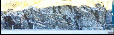
FACETS was applied to a 3D point cloud of road section located in Mannsverk, a suburb east of the city Bergen, Norway (5.3683°E; 60.3571°N). The outcrop faces west with a crudely north-south trend. The rock is an “amphibolite, transformed and severely deformed gabbro and green stone with bands of trondhjemite” (NGU, 1/50.000 geological map). The outcrop is 20m long and 4m high.
Figure 1. Mannsverk outcrop, 20m-wide, 3-m-high, North is to the left, the outcrop is facing West. The geological scan line was surveyed slightly above the hand rail, from this perspective.
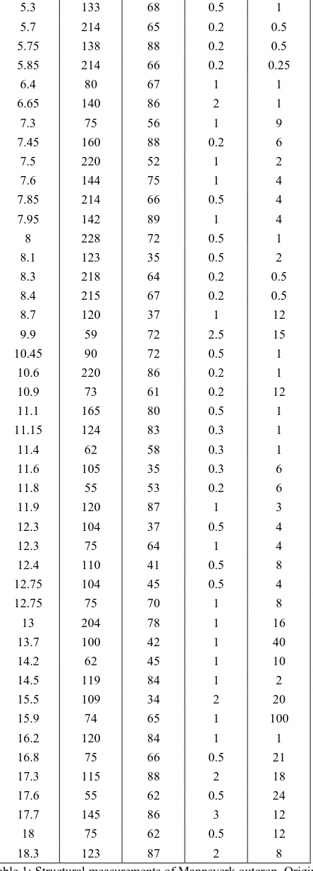
Following common geological practice, a 15-m-long scan line was established at a height of about 1.70m above the ground to systematically measure all planar facets being intercepted by this line. 59 structural measurements were performed reporting approximate linear coordinate of the facet centroid along the line, the strike and dip of the facet, its eye-balled roughness amplitude and approximate surface area (Table 1). This is the explicit population, from a field geologist’s judgement, of all the planes expressed in the outcrop at this height. To ensure correct correspondence between field measurements and 3D cloud computation, each facet was labelled with silver-gray duct tape stuck onto the rock face with compass/clinometer readings prior to shoot the photographs.
Four main families of planar facets appear from compass measurements (dip direction use clock-wise rotation down-to-the-right convention): east-pointing steep N075°E/60° and shallow N110°E/40°; south-east pointing N150°E/87°; and south-west point N210°E/65°.
Linear coordinat
e [m]
Dip direction
[°]
Dip [°]
Apparent roughness amplitude
[cm]
Estimated surface area [dm²]
2.7 90 14 0.5 16
3.1 178 76 2.5 12
3.3 86 66 0.5 18
3.6 171 85 2.5 18
3.8 255 35 1 8
3.9 165 85 0.5 2
4.1 160 86 0.5 2
4.2 160 85 0.5 3
4.6 45 62 0.2 2
4.9 120 64 0.2 0.5
5 195 56 0.2 0.5
5.1 130 64 1 1
5.15 204 56 1 1
5.23 220 52 0.5 0.5
5.3 133 68 0.5 1
5.7 214 65 0.2 0.5
5.75 138 88 0.2 0.5
5.85 214 66 0.2 0.25
6.4 80 67 1 1
6.65 140 86 2 1
7.3 75 56 1 9
7.45 160 88 0.2 6
7.5 220 52 1 2
7.6 144 75 1 4
7.85 214 66 0.5 4
7.95 142 89 1 4
8 228 72 0.5 1
8.1 123 35 0.5 2
8.3 218 64 0.2 0.5
8.4 215 67 0.2 0.5
8.7 120 37 1 12
9.9 59 72 2.5 15
10.45 90 72 0.5 1
10.6 220 86 0.2 1
10.9 73 61 0.2 12
11.1 165 80 0.5 1
11.15 124 83 0.3 1
11.4 62 58 0.3 1
11.6 105 35 0.3 6
11.8 55 53 0.2 6
11.9 120 87 1 3
12.3 104 37 0.5 4
12.3 75 64 1 4
12.4 110 41 0.5 8
12.75 104 45 0.5 4
12.75 75 70 1 8
13 204 78 1 16
13.7 100 42 1 40
14.2 62 45 1 10
14.5 119 84 1 2
15.5 109 34 2 20
15.9 74 65 1 100
16.2 120 84 1 1
16.8 75 66 0.5 21
17.3 115 88 2 18
17.6 55 62 0.5 24
17.7 145 86 3 12
18 75 62 0.5 12
18.3 123 87 2 8
Table 1: Structural measurements of Mannsverk outcrop. Origin of linear coordinates is arbitrary. Dip direction convention follows compass clockwise rotation (as in Nxxx°E) aimed so with the down-to-the-right rule.
3.2 3D point cloud SFM acquisition
The Mannsverk outcrop (Figure 1) was surveyed by means of Structure-from-Motion (SFM) technique, following recommendations by Wenzel & Rothermel (2013), among which: (i) keep short baselines between view-points (B/H ratio typically 0.2); (ii) shoot a panorama, from left to right, at every station to include oblique to outcrop line-of-sights; (iii) use a wide-angle lens for the same purpose; (iv) document overall outcrop (photos from afar) then shoot closer views for details. Watch out for harsh shadows and prefer even lighting (either somewhat veiled sun or even shadow exposure). Photo stations were performed in three parallel lines, 20m-away, 5-m-away and 2.5-m-away with the camera aiming horizontally. No additional shots were taken looking up from a low vantage point, nor down from a higher vantage point. The validation data set was acquired at man’s height, so at least those facets will be appropriately reconstructed.
A set of 124 photos were shot with a Nikon D7000 (4928x3264=16Mpix, APS-C 23.6x15.7mm, pixel pitch 4.79µm) equipped with Sigma 20mm f/1.8 fixed focal length. Georeferencing was performed with Solmeta Geotagger Pro-2, but outcrop scaling used quadrants targets distances among them were surveyed by laser range finder. Vertical of the site was established at both ends with vertically aligned quadrant targets, 2.1m and 2.6m apart. Vertical alignment was performed with LEICA Lino2 laser level. Equipments brands and types are referred to for technical specification purposes, not as commercial endorsement.
Outcrop azimuth trend is related to a reference direction materialized by two targets on the ground, 5.1m apart and compass reading. Although not perfect, an EDM-total-station will be far more accurate; this SFM survey conforms with light-weight constrains geologist will use in the field. Vertical established by self-levelling laser is vertical within 2.10-4 rad (±1mm/5m) (note the markers left and right of Figure 1, two on the wall to the left, two on the lamp-post on the right).
The point cloud was computed with Agisoft Photoscan v1.2.3. 124 photos were used for alignment and bundle optimization entering target-to-target distance constrains, and removing spurious sparse points (gradual selection of points appearing on only 2 photos and manual clean-up of obvious blunders). Two dense point clouds were generate, one with “medium mild filtering” and the second with “high density, mild filtering”. Only the second was retained for further analysis (see discussion below). Both were generated with the two closest shooting station rows. Very few blunders came out in the processed, which were cleaned out.
The point cloud contains 39.6 Mpts. 31.3 Mpts belong to the outcrop. A subset of 9Mpts was sampled as a 1m-high band across the scan line survey area. Half the points of the area of interest lie closer than 2.4mm (median point spacing), while 99% of points are closer than 4.5mm. For initial representation purposes, normals with a radius of 4mm were computed for each point (Figure 2).
Figure 2. 3D RGB point cloud with a 1m-high area of interest around the scan line survey where normal are colored by HSV.
3.3 FACETS segmentation
Facet computation was performed on the scanline point subset. A set of 4 well identifiable facets in 4 different orientations were manually sampled to assess realistic maximum distance (see 2.6). 68% of points lied within 6mm of their respective best fitting planes. This was used as Q68% maximum distance. Maximum angle was set to 10° as these could be discriminated in the field. 100pts were deemed minimum for declaring a facet. This threshold was observed to be realistic in the field where the smallest sampled facet was 5x5cm² (>120pts if points happened to be surprisingly sparse). These setting produced 7984 facets (Figure 3).
Figure 3. Facets extracted around the scanline. Colours depict normal with HSV convention (Hue assigned to dip direction).
3.4 Comparison of results
At the outcrop scale, a very large number of facets were extracted, which makes it difficult to review here. A more synthetic view is offered with the stereogram (Figure 4).
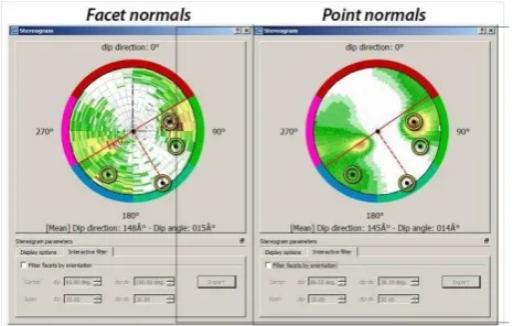
Figure 4. Stereograms of facets (left) and of point normal. Circles represent the dominant families surveys along the scan
line.
The stereogram of facet normals appears patchy (Figure 4, left), this is because points are classified into discrete values. On the right, the stereogram of 3D points with normal computed at 4mm radius. This representation is far more continuous and makes it easier to discern dominant features. On both, the dominant families intercepted by the scan line are plotted with their dispersion. It appears that the scan line explicitly recognized the N075°±20°/60°±20°; while the point normal stereogram (Figure 4, right) shows that it is rather focused on N085°E±30°/55°±30°. With such dip and dip direction range, the second mapped family actually falls on the edge of this primary peak.
The other three dominant families mapped with the scan line, seem to have come across rather conspicuous facet attitudes. When sounding the point cloud for the apparently absent pole at N150°E±30±/85°±10°; a series of points do in fact come out. Their number however is really limited for the surface area they represent on the outcrop is confidential. The white shade of stereogram colour ramp, which is customizable, is somewhat deceptive in this case. Yet it is difficult to design a colour ramp capable of bringing discrimination both with very high and very low density values. And currently, there is no option to modify the density scale with transforms such as log density, to squeeze extremely large peaks and bring them into a narrow range of values.
4. DISCUSSION
FACETS appears to have performed well to map explicitly the entire outcrop. A facet-by-facet check was undertaken, which showed good agreement to within 10° of both dip and strike of digital versus compass/clino mesurements. This is not surprising as natural outcrop roughness explains such variability. Beyond this check, the stereogram synthesis shows how compass measurements and scan lines do not reflect the same information as 3D point clouds. Figure 4 shows that the outcrop is largely dominated by specific orientations. But when accounting for them in a weighted manner, i.e. resuming several hundred thousand points as one patch of contiguous plane, other orientations appear (Figure 4 left). The dominant directions, green and blue areas visible on Figure 2, are made of single large planes. They are bound to host many 3D points as they occupy the largest portion of the outcrop. Fractures entiring the outcrop (red narrow nearly vertical fractures oriented N045°E±20°/85°±20°) have very small footprint on the outcrop and pass mostly unnoticed.
Are SFM point clouds appropriate for mapping geological structures at outcrop scale? As mentioned above, dense cloud parameter to “medium”, which is practical with respect to computing time, corresponds to dividing original pixel count by 16 (image width and height each divided by 4). This is equivalent to turning a 16Mpix detail rich photo into a crude 1Mpix image. In this case study, photos included in the dense cloud generation were shot 5 and 2.5m away from the outcrop. At 5m, the furthest shooting distance used, the image to object scale is 1/250 (focal length/distance: 20/5000, both expressed in mm). For a pixel pitch of 4.79µm, this scaling factor produces ground sampling distance of 1.2mm. When resampling original images, this ground sampling distance at “medium density” becomes 4.8mm. This value may still acceptable for many purposes, but should really take into account which geological features are expressed in the outcrop. The smallest facets surveyed in the scan line have a surface area of 5 x 5cm². Point cloud models should really try and retrieve a sufficient amount of points to map them with precision.
Lower point density in dense cloud extraction not only reduces the ground sampling distance, which may be detrimental to small facets, but also smoothes their edges. Such edge effect reduces the apparent sharpness of otherwise known sharp edges in the field and biases visual inspection. But further, smoothed edges curve the surface and pull edge points away from the best fit plane. This will affect plane attitude estimates. Perhaps an indication of density is to ensure that ground sampling distance is sufficient to preserve 80% of the facet central part unaffected by edge effect.
This edge effect discussion calls for another comment. FACETS segments point clouds into planar objects with algorithms that cluster elementary planes into larger objects using a complanarity indicator and a roughness criterion. The outcome is bound to have an infinity of realizations. This algorithmic approach is however valid for reaching an interpretation consensus, as all field experts may agree easily on what makes a planar facet core area. Early work of Dewez 2003 presented in Dewez & Stewart, 2015 focused on this mapping consensus issue. Finding edges that reach a broad consensus is near to impossible. Every expert will apply a different rule, and true geological facets often blend into another feature seamlessly. While some facets have clear and sharp edges (see the work of Vasuki at al., 2014), many do not. The plugin FACETS implements one possible realization of point cloud segmentation and makes it available to the community.
Geologists should not turn a blind eye to field outcrops, nor fear that 3D cloud will replace fieldwork. There are situations where a compass/clinometer cannot be replaced. When the planar features of interest are not expressed as measurable surface, point clouds do not contain any relevant information. Stratification planes in shallow dipping monocline settings often occur as thin elongated ledges. Point clouds may not represent them well firstly because their width are not well sampled by points, and secondly because the points of view to acquire them adequately may not have been chosen when surveying, possibly even for field good reasons. Virtual outcrop geology is a very advantageous tool for many applications but does not replace fieldwork.
5. CONCLUSION
FACETS is plugin for planar facet extraction available in
CloudCompare as of v2.6.2
http://www.cloudcompare.org/doc/wiki/index.php?title=Facets_ %28plugin%29. It implements elementary planar object recognition with minimal user input. Elementary planar Facets recognized either through Kd-Tree or Fast Marching algorithms are grouped into planes and families. FACETS provides a graphical user interface to represent stereograms of objects with normals attached, be them planar vectorial facets or even point clouds with normals. The stereogram dialog box offers both numerical and interactive query functionality to see selected objects in 3D space. Beyond strict geological application, these queries prove very practical for segmenting architectural and underground mine/quarry point clouds.
This paper presents a test where field structural geology data was collected on a scan line and compared with digitally processed 3D point clouds. A scan line turns out to reduce the amount of geological information drastically (too drastically). Structural analysis of 3D point cloud on the other hand will be overwhelmed by the planar facets occupying the largest surface area. Implementation of the interactive stereogram proved very practical to explore the dataset and segment it. Such segmentation is amenable to further computation such as fracture spacing.
ACKNOWLEDGEMENTS
The development of FACETS was supported financially by BRGM internal project DEV-ESCARP. Field data collection in Mannsverk was financially supported by BRGM’s Carnot Institute mobility projet RADIOGEOM. TD wishes to thank
Benjamin Dolva from the Virtual Outcrop Group CIPR (UniResearch) for assistance in field data collection.
REFERENCES
Assali, P., Grussenmeyer, P., Villemin, T., Pollet, N., Viguier, F., 2016, Solid images for geostructural mapping and key block modeling of rock discontinuities, Comp. & Geosci., 89, 21-31,
http://dx.doi.org/10.1016/j.cageo.2016.01.002.
CloudCompare (version 2.6.2) [GPL software]. (2016). Retrieved from http://www.cloudcompare.org/
Dewez, TJ.B., 2003, Geomorphic markers and digital elevation models as tools for tectonic geomorphology in central Greece, PhD Thesis, unpublished, Brunel University, Uxbridge, United Kingdom, 194p.
Dewez, T.J.B., Stewart, I.S., 2015, From Digital Elevation Models to 3-D deformation fields: a semi-automated analysis of uplifted coastal terraces on the Kamena Vourla Fault, central Greece, in Dykes, A.P., Mulligan, M., Wainwright, J. (eds.),Monitoring and modelling Dynamic Environments, Whiley Blackwell, London, 226-247.
Fernandez., O., 2005, Obtaining a best fitting plane through 3D georeferenced data, J. Struct. Geol., 27, 855-858.
Riquelme, A.J., Abellán, A., Tomás, R., Jaboyedoff, M., 2014, A new approach for semi-automatic rock mass joints recognition from 3D point clouds, Comp. & Geosci., 68, 38-52,
http://dx.doi.org/10.1016/j.cageo.2014.03.014.
Vasuki, Y., Holden, E.-J., Kovesi, P., Micklethwait, S., 2014, Semi-automatic mapping of geological Structures using UAV-based photogrammetric data: An image analysis approach,
Comp. & Geosci., 69, 22-32,
http://dx.doi.org/10.1016/j.cageo.2014.04.012
Wenzel, K., Rothermel, M., Fritsch, D., Haala, N., 2013, Image acquisition and model selection for multi-view stereo, Int. Arch. Phot. Rem. Sens. & Spat. Inf. Sci., XL-5/W1, 25 – 26 Feb. 2013, Trento, Italy
Revised April 2016