A NEW IDL IMPLEMENTATION OF THE JUPP METHOD FOR BATHYMETRY
EXTRACTION IN SHALLOW WATERS
M. Deidda a, A. Pala a, G. Sanna a
a DICAAR, University of Cagliari, 09123 Cagliari, Italy - (mdeidda, apala, topoca)@unica.it
Commission VII, WG VII/5
KEY WORDS: Bathymetry, Remote Sensing, Coastal Erosion, IDL
ABSTRACT:
There is an ongoing effort in using imagery from remote sensing platforms to obtain information about the sea depth; this allows to monitor the dynamics of coastal erosion without the need for costly and repeated local surveys. We worked on a new implementation of the Jupp method to extract depth information from satellite images. Our software is based on previous implementations of the algorithm in the IDL language, but we made our current implementation more modular in order to make possible experimentations with different approaches. We used this implementation on a series of six images (three from the Landsat TM sensor and three from the Landsat OLI sensor) in order to improve the available tools. We established an iterative workflow for working on the Landat-8 images widely exposed in this paper.
1. INTRODUCTION
The availability of high resolution satellite images makes remote sensing an attractive approach to the problem of determining sea depth in coastal areas. This is especially promising in the field of coastal erosion monitoring and management that would otherwise require costly and extensive bathymetric surveys. In order to exploit this resource, many recent satellite platforms are equipped with a specific “coastal” sensor, which is sensitive to a slightly higher wavelength than the usual blue band. Such wavelengths have a better water penetration, thus allowing to extend the bathymetry estimate to grater depths.
Since the 1980s, there have been many studies on the subject of extracting bathymetric information from remote-sensed imagery, both regarding experimental procedures and software implementations. For the purposes of our research, we built our own implementation of the Jupp algorithm in the IDL language, which allows us to take advantage of the ENVI platform by Exelis-VIS performing the preparation of input data, visualization and comparison of the results.
Thanks to the USGS EarthExplorer project we had access to recent Landsat-5 and Landsat-8 imagery of Sardinia which were used as dataset for testing and analysis purposes. We used three scenes from the Landsat-5 satellite (using the TM sensor) and three from the Landsat-8 (using the OLI sensor), arranged into two chronological sequences.
After a brief historical review, the algorithm, the software and the results on Landsat images are presented in the following paragraphs.
2. STATE OF THE ART
2.1 Methods for bathymetry information extraction
The principle underlying the use of remote sensing for determining bathymetry is that different wavelengths of light penetrate water to different depths.
When passing through water, light is attenuated as a consequence of its interaction with the water column. The intensity of the light after crossing water for a length p is
��= � −�� (1)
where I0 is the intensity of incident light and k is the attenuation
coefficient, which is dependent on the wavelength of the incident radiation.
If we assume that the path of light from the surface to the bottom and back is vertical, then the distance p can be replaced with 2d, where d is the water depth. Linearizing the previous expression we obtain:
ln �� = ln � − 2 � (2)
In the visible part of the spectrum the electromagnetic radiation with the grater wavelength (red) has a greater attenuation coefficient than the one with smaller wavelength (blue). The depth of penetration also depends on the turbidity of the water: sediments in suspension, phytoplankton and dissolved organic particles affect the penetration capacity by producing absorption and diffusion effects, and thus limiting the range in which the radiance data can be used to evaluate the water depth.
The models that apply the concepts exposed here and allow to extract bathymetric information from satellite imagery are essentially three: the Benny and Dawson method, the Lyzenga method, and the Jupp model, also known as the DOP (Depth Of Penetration) Zones method.
The Benny and Dawson method adds to the ideal path a single correction, defined only in geometric terms, to compensate for the fact that the Sun is not vertically overhead at the time of image acquisition (Green, 2000).
The Lyzenga method, like the others, works on the assumption that the attenuation of light is an exponential function of the water depth and that the quality of water does not vary across the image; for that reason, the ratio (ki/kj) between the coefficients of
attenuation in different bands (i, j) of the same image must be constant. The relative depth can thus be deduced from the position of the pixel on the ki/kj regression line, considering that
The Jupp method is based on the concept that for every band in the image there is an area where only the corresponding wavelength can penetrate to the bottom and then back to the surface in order to be detected by the sensor. In that specific area, that wavelength gives the best depth information, because the signal is neither too weak nor too saturated. The method thus identifies a Depth Of Penetration Zone for each band, and then deduces the depth inside each DOP zone by applying the equation (2).
Regarding the Benny-Dawson and Lyzenga methods, the literature (Green, 2000) reports that the correlation values between calculated and measured depths, for a site with water characteristics comparable with the case here presented, are too low to recommend their use for the purpose of estimating depths. Conversely, the same studies report much higher correlation values for the Jupp model, up to 0.9 for the calibrated model. The algorithm and its implementation are described in the following paragraphs.
2.2 Previous works using the same method
Gianinetto et al. (2004) applied the general principle of the Jupp method to QuickBird imagery of the Lagoon of Venice, but had to contend with the fact that water in the area is rich in sediments and is considerably spatially variable in transparency. They approached the problem by introducing a parameter in the equation (3) to account for this local variation, and then modelling this parameter with a genetic algorithm. In practice, their algorithm models the different transmission of light in each layer of the water column by trying different solutions and choosing the one that more closely aligns with the sample data. The results had correlation values usually between 0.65 and 0.94. Nguyen et al (2007) applied the Jupp method to Landsat-7 ETM+ imagery of an area in the Vietnam Sea (Ly Som Island), taking the depth sample points and control points from a marine chart. They obtained a 0.76 correlation coefficient between the results of the algorithm and the control points, which they deemed not good but promising. In Deidda (2008) the method was applies to an area in Sardinia (Italy) using both Landsat TM5 and Ikonos imagery. The depth sample points and control points were provided by an echo-sounder bathymetric survey. Applying the algorithm to the Landsat TM5 image, the results showed a correlation coefficient of 0.76 comparing the estimated depths with the control points. For the higher resolution Ikonos image it was necessary to perform a preliminary classification step in order to divide the image in areas of uniform benthos. A further implementation to a WorldView 2 stereo pair, reported in Deidda et al. (2012), shown precision of about 0.6 m.
3. THE JUPP METHOD
3.1 General model
According to the model revised by Jupp in 1988, the following three hypotheses must be verified:
1. Light attenuation is an exponential function of depth. 2. The quality of water (and thus the coefficient of
attenuation k) does not change inside the image. 3. The albedo of the sea bottom is almost constant in the
image.
The third condition can be assured by first performing a bottom classification, and then applying the method separately to each habitat.
The application of the Jupp model is divided into two phases: 1. Determining the DOP zones:
2. Interpolating the depths inside each DOP zone.
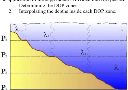
Figure 1. Penetration of light in water depending on wavelength.
3.1.1 Determining the Depth Of Penetration Zones: the DOP zones are defined by the maximum depth of penetration of each wavelength. Even at a greater depth with respect to the other bands the blue band will present some bottom reflection, because the shorter wavelengths penetrate better the water column, thus getting a light signal back to the sensor.
The attenuation of light through the water column was modelled by Jerlov (1976) and later recalculated by Jupp (1988). The maximum depths of penetration in the four bands of the Landsat TM5 sensor are reported in the following table 1 as in GREEN, E. P. et al, 2000.
Table 1. Maximum depth of penetration by band
Considering the water column and a sensor where the energy of the light ray is separated into blue, green, red and near infrared components, and specifying with λ1, λ2, λ3and λ4 the respective
wavelengths for each channel, we’ll have that the wavelength λ1
will penetrate down to the depth P1, the wavelength λ2 will
penetrate down to the depth P2, λ3 down to P3, and λ4 down to P4.
The Jupp model applies these concepts translating them into the determination of depth bands, or DOP Zones, each of which allows an estimation of depth according to the attenuation undergone by the light in the corresponding wavelength. From this follows that it’s possible to apply the algorithm to imagery produced by those satellite sensors which cover this range; many medium and high resolution sensors satisfy these requirements.
The depths in table 1 are meant to be coarse values. In order to better estimate absolute depth values it is necessary to perform in situ depth measurements in a number of sample points, in the area covered by the image. This is necessary because the water column might have different optical characteristics depending on its temperature, salinity, and amount of substances in suspension.
perceived by the sensor will be determined for each band. The maximum (LbM), minimum (Lbm) and mean (Lbd) values of the pixels in this sample region are then calculated for each band b.
Afterwards, each of the depth sample points is associated with the DN of the corresponding pixel in each band. In order to avoid image pixel interpolation the image reference frame is assumed valid and the sample points are referenced in the image frame. For this, the sample points coordinates are converted in pixel coordinates.
Starting with band 1, corresponding to the blue band, the sample points are sorted in order of decreasing depth, and consequently the corresponding DNs will be sorted in increasing order. The value of L1M behaves as a threshold that divides the DNs into two sets: the set D1 containing the sample points whose DNs are lesser than L1M, the set D2 containing the points whose DNs are equal to L1M and the set D3 containing the points whose DNs are greater than L1M. This partition can be done even if there is no point in the sample whose DN corresponds exactly to L1M, this because its value will fall between the DN value immediately greater than L1M and the DN value immediately lower than L1M in the sample; in this case the set D2 will be empty. The depth z1 (the maximum depth where signal is returned from the sea bottom in the blue band) is then calculated as the mean of the average of the depths of the points in D2 and the average of the depths of the points in D3.
In order to improve this estimation, the depth values higher than
z1 but with a DN greater than L1M and those with depth lower than
z1 but DN lesser than L1M must also be considered. In our implementation, we considered D1 and D2 as a single set, and used its average depth in the calculation of z1.
By repeating this procedure, we obtain the depth limit zb for each band b.
From the combination of the threshold values thus defined and the maximum DNs of the calibration zone, the method then defines the rules according to which each pixel will be assigned to a specific DOP zone only. In fact, the zones are defined according to a principle of mutual exclusion, even if there might be response from more than one band. The pixels whose DN values are lesser than the maximum value of the calibration area for the correspondent band (LbM) will have a depth greater than the maximum penetration depth for that wavelength.
3.1.2 Interpolation of each DOP Zone: Remembering that algorithm in the IDL 8.2 language, in order to use it together with the ENVI 5.0 visualization software.
The routines are based on the code presented in Deidda (2008) and incorporates part of it. In this new implementation, the main program is a graphical user interface in which the operator can perform the various steps of the algorithm in a predefined order while checking for intermediate results.
2. Selection of the deep water values a. From a sample area b. From direct input 3. Calculation of the DOP zones
4. Determination of the maximum depth zb of each DOP zone
a. From a file of sample depths b. From direct input
5. Interpolation of the depth values
Steps 2 and 4 can be performed using the outcomes of the Jupp algorithm, otherwise the operator can supply alternative values. The results of steps 3 and 5 can be previewed in separate windows, saved on disk, and/or exported to the ENVI software for further processing.
4.1 Input Data and Project File
possible to edit the subset coordinates manually. Lastly the land mask image is selected in a standard image selection dialog; in this case a single band is considered and it's not possible to define a subset (the same subset as the input image is used).
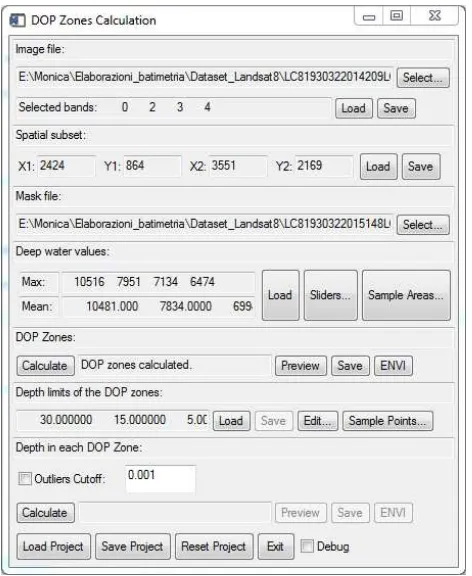
Figure 2. Main program interface
The user can save all the settings related to the input data into a "project file" which can later be loaded so as to make different calculations with the same input data. At this stage, the "project file" does not contain the intermediate results of the calculations; this choice was made because the routines related to the algorithm are still a work in progress, and it would make little sense to save the results of superseded versions of them.
4.2 Deep-water values
This section controls the routines that estimate the representative values of deep water (i.e. beyond the penetration ability of that wavelength) for each band. In particular, as explained in 3.1.1 and 3.1.2, we need the maximum DN of a deep-water area (LbM) in order to define the DOP zones, and the average DN of the same area (Lbd) in order to interpolate the depths inside each DOP. Based on our experience we developed two different tools, "Areas" and "Sliders".
The former, “Areas” is a direct implementation of the Jupp algorithm. This command opens a new window, which shows an interface for selecting rectangular areas and calculating their maximum and average values in each band. The areas are drawn as rectangles on a scaled-down view of the area of interest. In order to better find the deep-water areas, it is possible to switch from the natural colours view (RGB bands) to a false-colours view of the blue band only (because the blue intensity is the last one to decrease as the depth increases). The user can select multiple rectangular areas on the working subset, activate and deactivate each of them, and see the resulting maxima and averages in real time. This means that it is possible to have an immediate preview of the DOP zones as the deep-water area is
selected. The user can load and save the list of areas for later use. If none of the selected areas gives good results, it is possible to discard the entire list and start from scratch. Once the deep-water values have been calculated, they are saved to a file. The deep-water sample area may be of any size. It is also possible to calculate values from areas which are the union of multiple rectangles.
In the latter tool “Sliders” the user can directly modify the deep -water values by typing them in input boxes (both maxima and averages) or by means of sliders. Here too it is possible to preview the results of the chosen values and save them to a file.
The main program interface also contains a button to load the deep water values produced with the two methods. This allows for example to calculate the deep water values on a portion of the image, and use them in a different portion.
Note that in this version of the software, the coordinates of the sample areas are pixel offsets relative to the current subset. On one hand, it could be useful to retrieve the map coordinates of the sample area for reference purposes. On the other hand, our tests suggest that the location of the best sample deep water area depends on the specific image due to the different lighting and water conditions; it's generally not possible to reuse the location of an image's sample area for a different image.
4.3 DOP Zones Calculation
This section activates after the deep water values are determined (with any method), and launches the calculation of the DOP zones. The calculation routine is generalized in order to be usable with any number of bands. Also, rather than a binary DOP mask for each band, this routine outputs a bitmap where each pixel value corresponds to the number of the DOP zone it belongs to, or 255 if it is not in any DOP zone. (255 is used as the "no zone" value because 0 is a valid band number and thus a valid DOP zone identifier.) Masked pixel of course are also set to 255. This encoding means that the bitmap, with an appropriate color table applied, can be used to visually show the different DOP zones.
Once the DOP map is calculated, more buttons activate: they allow previewing the map in a separate window, to export it to a file, and to export it to the ENVI software where it can be overlaid on the input image for visual inspection. The saved image is georeferenced (based on the geographic metadata of the original image), thus DOP maps calculated from different images can be overlaid and compared.
4.4 DOP Depth Limits
This section is related to the determination of the maximum depth of each DOP zone (zb). Once again, the user has a choice: manual input, or calculation based on sample points. Manual input can be used to check the result on the algorithm when using standard values. Alternately, the program can read a text file containing a series of sample points (each described in coordinates and depth) and calculate the depth limits as described in 3.1.1.
Like the deep-water values, the depth limits can be saved to a file to be reused in later calculations.
4.5 Depth Values Interpolation
option to use a lower threshold for � � by cutting the highest DN values; it can happen that the highest DN values occur only in a small number of pixels and thus do not make a statistically significant sample. The program produces a double precision floating point matrix encoded as a raster image.
After the calculation is performed, the depth image can be previewed in a new window, saved to a file, and/or sent to the ENVI software for further processing.
4.6 Final notes
The software was not designed as a product for final users, but like a laboratory where researchers can experiment with different combinations of parameters and procedures. For this reason, there is also a "debug" switch that enables the production of additional (and very verbose) information on the IDL console.
5. EXPERIMENTATION
5.1 The Data Set
5.1.1 For the purposes of this research, we used the Landsat sensors because they responded to several requirements. As we wanted to test the Jupp method in its “raw” form, we chose a medium-resolution sensor that would not need pre-processing operations (e.g. sea bottom classification). Moreover, images from Landsat sensors are available and free of charge for end users. All the imagery used in this study were downloaded via HTTP from the USGS EarthExplorer interface (USGS 2015) after registering to the site.
We considered two temporal series, one for the TM5 sensor and one for the OLI sensor. Table 2 summarizes the characteristics of each sensor and scene, extracted from the respective metadata,
Table 2. Characteristics of the scenes
Table 3 instead summarizes the characteristics of the used sensors.
Band designations
Landsat band wavelength comparisons All bands 30-meter resolution unless noted
L8 OLI/TIRS L4-5 TM
T1 = Thermal (acquired at 100 meters, resampled to 30 meters) T2 = Thermal (acquired at 120 meters, resampled to 30 meters)
Table 3. Landsat band wavelength comparisons
The series using the TM5 sensor covers a range of acquisitions of six years; the one based on the OLI/TIRS sensor covers a much shorter interval of two years. In choosing the images we also paid particular attention to the quality and the cloud cover on the sea areas. We chose not to use images with a quality parameter lower
than 7 (the quality parameter ranges from 0, the worst, to 9, the best). Where there was cloud cover over the sea, it was masked together with the land areas and excluded from the calculations. All the scenes were acquired in a descending orbit.
All the downloaded images present an L1T processing level. This means that the product delivered to the end user is a radiometrically and geometrically corrected image. The image is georeferenced in the WGS84 reference system and orthorectified using the GLS2000 data set as reported in Landsat Thematic Mapper Level 1 data format control book (DFCB) (USGS 2015). The Global Land Survey (GLS) data sets were designed to allow scientists and data users to have access to a consistent, terrain corrected, coordinated collection of data. The level one image is presented in units of Digital Numbers (DNs) which can be easily rescaled to spectral radiance or top of atmosphere (TOA) reflectance.
5.2 Landsat 8 analysis and processing
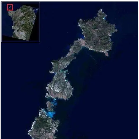
For the Landsat 8 images, we used a subset including the Asinara Island in north-western Sardinia (Italy).
Figure 3. The Asinara island (Italy) and its position with respect to Sardinia.
The bands used were 1 (Coastal), 3 (Green), 4 (Red), 5 (Near Infrared). Despite of the images covering almost the same area and being georeferenced in the WGS84 system, the landmask was recalculated for each image because of the different cloud covers and slightly different dimensions. The landmasks were obtained first with an automated procedure and then edited manually to clear masked areas that should have been left unmasked and mask cloudy areas that the automated procedure had not masked.
general bathymetry of the area as known by other sources until we found for each image the area that gave the best results.
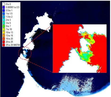
Figure 4. Various deep water sample areas, and the DOP zones resulting from using one of them.
At this point we calculated the DOP zones, which correspond to the preview in the area selection tool.
The results of the calculation are shown in Figure 5. Figure 6 shows the DOP zones calculated on the whole image with the same parameters. Note that the selected “deep water” area produces plausible results on the west coast of the island, but not on the north-eastern coast where the infrared DOP zone extends far further than is physically possible.
Figure 5. Results of the DOP zones calculation on the selected area.
Figure 6. DOP zones calculated on the whole image.
Since we don’t have depth sample points for this scene, we interpolated the depth values using the limits for the DOP zones as indicated in Table 1.
Figure 7. Depth images calculated on the scene acquired in 2013.
We then repeated the procedure for the other two Landsat-8 scenes. The results, put in chronological sequence, are shown in Figure 7, 8 and 9.
5.3 Landsat 5 analysis and processing
Figure 8. Depth images calculated on the scene acquired in 2014.
Figure 9. Depth images calculated on the scene acquired in 2015.
Like in the Landsat-8 case, for the Landat-5 scenes we started with selecting the “deep water” areas with the corresponding procedure. Unfortunately, in this case it was impossible to find an area that would give acceptable results. For this reason, we used the slider-based procedure to adjust the calculated maximum DN values by one or two units until the results were consistent with our knowledge of the area.
The difference between Figures 10 and 11 shows how by increasing by two DN units the value for Band 2 we changed the extension of the corresponding DOP zone. This operation would not be possible just by selecting sample areas.
This is the limit of the analysis that can be performed based purely on the images; in order to decide which value of the sliders produces the DOP zones that better match the actual depths, we should perform an actual bathymetric survey of a number of sample points.
Figure 10. Adjusting the maximum “deep water” values with the sliders interface.
Figure 11. Adjusting the maximum “deep water” values with the sliders interface.
5.4 Comparisons
Not having access to a series of bathymetric surveys or digital depth models that were consistent with the acquisition times of the images, we can only perform a comparative analysis of the sea bottom profile based on the theoretical depth penetration values. The resulting values thus don’t represent the actual depth values. Despite this, the fact that the images were calibrated and processed with the same parameters allows us to compare them for variations.
In an exercise that had the purpose of testing the correct behaviour of the algorithm, we applied the process to the three Landsat-8 images representing the same area in three successive years. We could not use Landsat-5 images in this comparison because at this point we wanted to test the algorithm using the “Coastal” band which that sensor does not support.
These conclusions are supported by the statistical analysis shown in the following graphs. Figure 12 shows the histogram of the difference between the 2014 and 2013 depth maps; we can see that the average difference is 3.78 m and the standard deviation is 4.82 m. Figure 13 shows the corresponding histogram for the difference between 2015 and 2014, where the average difference is -0.40 m and the standard deviation is 3.11 m. The differences have been calculated on those cells whose depth was determined in all three images.
Figure 12. Histogram of the difference between the 2014 and 2013 depth maps.
Figure 13. Histogram of the difference between the 2015 and 2014 depth maps.
6. CONCLUSIONS
In this work we started from previous research about the Jupp method and its application to produce a new implementation in the IDL language. We reconstructed the software as a tool a researcher can use in order to test the algorithm with different parameters. We used the software on two temporal series of three Landsat images each, the first from the Landsat-8 OLI sensor and the second from the Landsat-5 TM sensor. We calculated the DOP zones for both series and an indicative version of the interpolated depth for the Landsat-8 series. The comparison of the DOP zones in each series shows a coarse assessment of the variation of the sea bottom. A quantitative evaluation of the results will be possible with actual sample depth data for the area of interest.
We see this algorithm as a tool for small scale monitoring of a large coast extent such as the one of Sardinia.
The procedure is always iterative; starting with a coarse knowledge of the general bathymetry we can extract the DOP zones, and based on these we will plan a bathymetric survey. We can then use this information to refine the definition of the DOP zones, and so on. Once the DOP zones are well defined, the survey will provide the ground data for the interpolation of the depth values.
This method requires the calibration of the model through a bathymetric survey of the area of interest. For this reason we are designing and building a small ROV that will perform this operation.
We are also looking into the implementation of tools for comparing the results of different images, in order to have quantitative assessments of temporal series of images.
REFERENCES
BENNY, A. H., DAWSON, G. J., 1983, Satellite imagery as an aid to bathymetric charting in the Red Sea. The Cartographic Journal, 20(1), 5-16
DEIDDA, M., 2008. Impiego di immagini satellitari per il monitoraggio della dinamica costiera. 2008. Ricerche di Geomatica, AUTEC, pp.71-80.
DEIDDA, M., SANNA, G., 2012. Pre-processing of high resolution satellite images for sea bottom classification. Int J Remote Sens, 44.1: 83-95.
DEIDDA, M., SANNA, G., 2012. Bathymetric extraction using Worldview-2 high resolution images. International Archives of the Photogrammetry, Remote Sensing and Spatial Information Sciences, 39: B8.
GIANINETTO, T; Lechi, G, 2004. “A DNA algorithm for the bathymetric mapping in the lagoon of Venice using QuickBird multispectral data”. Conference: XXth ISPRS Congress, "Geo-Imagery Bridging Continents", Volume: The International Archive of the Photogrammetry, Remote Sensing and Spatial Information Sciences, XXXV(B), pp.94-99.
GREEN, E. P. et al, 2000. Remote Sensing Handbook for Tropical Coastal Management. Paris, UNESCO Publishing.
JERLOV, N.G., 1976. Optical Oceanography. Elsevier, New York.
JUPP, D.L.B., 1988. Background and extensions to depth of penetration (DOP) mapping in shallow coastal waters. Proc. Symposium on Remote Sensing of the Coastal Zone IV. Gold Coast, Queensland, pp. 2.1–2.19.
LYZENGA, D. R., Passive Remote Sensing techniques for mapping water depth and bottom features. Applied Optics, 17, 379 - 383
NGUYEN, T. K. N., LE, N. N., 2007. Bathymetry Mapping from Satellite Images for Ly Son Island, Quang Ngai Province. VNU JOURNAL OF SCIENCE, Earth sciences, T.xxIII, N01, pp. 51-58.
U.S. GEOLOGICAL SURVEY, 2015. Landsat Thematic Mapper (TM) Level 1 (L1) Data Format Control Book (DFCB), http://landsat.usgs.gov//documents/LSDS-284.pdf
U.S. GEOLOGICAL SURVEY, 2015. Landsat—Earth observation satellites: U.S. Geological Survey Fact Sheet 2015– 3081, http://dx.doi.org/10.3133/fs20153081.
U.S. GEOLOGICAL SURVEY, 2015. Landsat 8 (L8) Data Users Handbook Version 1.0. June 2015. http://landsat.usgs.gov//documents/Landsat8DataUsersHandboo k.pdf. Sep.
U.S. GEOLOGICAL SURVEY, 2015. USGS Earth Explorer.