PERFORMANCE ASSESSMENT OF INTEGRATED SENSOR ORIENTATION WITH A
LOW-COST GNSS RECEIVER
M. Rehak, J. Skaloud
´Ecole polytechnique f´ed´erale de Lausanne (EPFL), Switzerland - (martin.rehak, jan.skaloud)@epfl.ch
KEY WORDS:Sensor orientation, MAV, Lever-arm, Low-cost GNSS
ABSTRACT:
Mapping with Micro Aerial Vehicles (MAVs whose weight does not exceed 5 kg) is gaining importance in applications such as corridor mapping, road and pipeline inspections, or mapping of large areas with homogeneous surface structure, e.g. forest or agricultural fields. In these challenging scenarios, integrated sensor orientation (ISO) improves effectiveness and accuracy. Furthermore, in block geometry configurations, this mode of operation allows mapping without ground control points (GCPs). Accurate camera positions are traditionally determined by carrier-phase GNSS (Global Navigation Satellite System) positioning. However, such mode of positioning has strong requirements on receiver’s and antenna’s performance. In this article, we present a mapping project in which we employ a single-frequency, low-cost (<$100) GNSS receiver on a MAV. The performance of the low-cost receiver is assessed by comparing its trajectory with a reference trajectory obtained by a survey-grade, multi-frequency GNSS receiver. In addition, the camera positions derived from these two trajectories are used as observations in bundle adjustment (BA) projects and mapping accuracy is evaluated at check points (ChP). Several BA scenarios are considered with absolute and relative aerial position control. Additionally, the presented experiments show the possibility of BA to determine a camera-antenna spatial offset, so-called lever-arm.
1. INTRODUCTION
Unmanned Aerial Vehicles (UAVs) are gaining importance in the mapping and monitoring tasks of our environment. The employ-ment of UAVs is attractive in terms of cost, handiness, and flexi-bility, as they fill a gap between aerial mapping of large areas and local terrestrial surveying. When cm-level accuracy is required for derived geospatial products, the conventional (i.e. indirect) approach of sensor orientation does not deliver satisfactory re-sults unless a large number of GCPs is regularly distributed in the mapped area. This adds a significant cost to a project while be-coming impractical in difficult, or inaccessible terrain. For over-lapping imagery in block configuration, the need of GCPs can be principally alleviated through precise control of aerial-position (Colomina, 2007).
1.1 Bundle Adjustment with Aerial Position Control
ISO benefits from aerial, image, and possible ground data. It is a robust and efficient method provided proper conditions of suffi-cient image overlap. Under certain observability conditions, ISO allows system and sensor parameters (e.g. antenna offset, interior camera parameters) to be self-calibrated.
Apart from measurements of tie-features in image and object space, the observations and conditions of exterior orientation can be in-troduced into the adjustment. The number of GCPs can thus be reduced considerably, or under certain configuration may even be completely eliminated. The observation equation that models the relation between the imaging sensor and an antenna-phase centre, for which absolute position is derived, takes the known form:
Xm+vmX =X m
0 +Rmc (Γ)·A c+
Sm (1)
where
Xm is the GNSS-derived position for one epoch in a Cartesian mapping framem,
vmX is the vector of aerial position residuals, Xm0 is the vector of a camera projection centre, Rmc(Γ) is the nine-elements rotation matrix from
cameracto mframe parametrised by the traditional Euler anglesΓ = (ω, ϕ, κ),
Ac is the camera-GNSS antenna lever-arm, Sm is the possible positioning bias in the
GNSS-derived positions.
To reduce the influence of GNSS-positioning bias on aerial posi-tions, temporal differencing of the above equation can be used for two consecutive epochstiandtj, (Li and Stueckmann-Petring, 1992).
∆Xm(tij)+vm∆X=X m
0(tj)−Xm0 (ti)+ R m
c(Γtj)−R
m c(Γti)
·Ac (2)
1.2 Accurate Kinematic GNSS Positioning
capacity is principally dependent on the RTK engine of the em-bedded multi-frequency and multi-constellation GNSS receiver. The cm-level kinematic satellite positioning is reached through the differential processing of the carrier-phase data. For that pur-pose, having low noise of phase observations is as important as its continuity (limited number of cycle-slips), a number of mea-surements and their geometry, a distance to a base etc.; the rea-son for which manned airborne mapping employs almost exclu-sively multi-frequency receivers. The ambiguity determination through single-frequency observations is an attractive option as proposed in (Odolinski and Teunissen, 2016) due to an afford-ability of single-frequency receivers. Furthermore, the proximity to the base (e.g. <1-2 km) theoretically allows, in many MAV missions, single-frequency differential processing. On the other hand, the quality of phase observations is related to the number of aspects that are less favourable in small UAVs: the level of electromagnetic interference, the presence of vibrations and/or high platform dynamics. The receiver build is influential in terms of tracking-loop bandwidth, bit sampling, oscillator stability, and mutlipath reduction. In this respect, the usage of mass-market re-ceivers for precise aerial position control is difficult to generalise and the applicability of a specific setup needs to be evaluated em-pirically in an operational environment.
Regarding the use, low-cost, single-frequency GNSS receivers are typically employed in automotive industry and consumer elec-tronics. Their use in surveying is possible but often limited to static or low-dynamic applications, e.g. glacier movement or de-formation monitoring (Benoit et al., 2015). They have been tested on MAVs in several cases, e.g. in (Stempfhuber and Buchholz, 2011) or (Mongredien et al., 2016). However, their use for the purpose of accurate aerial positioning of aerial imagery in cm-level has not yet been assessed under real mapping conditions and particularly not on fixed-wing platforms. Overall the em-ployment of a single-frequency, low-cost GNSS receiver on MAV platforms is challenging for following reasons:
• Quality of receiver’s front-end,
• limited resources for signal sampling/tracking,
• limited band-with/acceleration under which the signal track-ing works,
• less channels for signal tracking,
• single-frequency and thus worse capability of resolving am-biguities,
• limited support for synchronisation - input and output tim-ing,
• usually no internal memory,
• lower sampling frequency, i.e.<10 Hz.
1.3 Methodology and Paper Structure
The presented test aims at investigating whether a low-cost (< $100) mass-market GNSS receiver can provide accurate, i.e. cm-level kinematic positioning, to contribute in ISO. Additionally, the aim is to test the ability to self-calibrate the camera-GNSS antenna lever-arm vector.
Section 2 presents the used equipment, specifically the MAV plat-form and its sensors. Furthermore, important mission parameters are summarised. The third section concentrates on performance
analysis of the low-cost receiver by comparing the camera posi-tions with those calculated from the survey-grade grade receiver. The fourth section is devoted to BA projects with aerial position control with absolute and relative observations derived from the two receivers. Last section draws conclusions from the conducted research work.
2. EXPERIMENTAL SETUP
2.1 Mapping platform
The drone used for this study is a custom made airplane equipped with the open-source autopilot Pixhawk (Meier et al., 2012). The wingspan is 165 cm and fuselage length 120 cm. The maximal payload capacity is around 800 g. The operational weight varies between 2200-2800 g and flying endurance is around 45 minutes. Thanks to is lightweight construction, the launching can be done by hand and it requires only a small place for landing. The plat-form’s main components are depicted in Fig. 1
Figure 1. Fixed-wing platform.
2.2 Sensor Equipment
The chosen optical sensor is the Sony NEX-5R camera (Sony, 2016). The quality of this mirror-less camera is comparable with a DSLR (digital single-lens reflex) camera despite being consid-erably smaller (only 111 x 59 x 39 mm) and lighter (290 g with-out lens). These properties make it highly suitable for MAV plat-forms. The camera is equipped with a 16 mm fixed Sony lens, which has a reasonable optical quality given its size and weight and offers sufficient stability of the additional distortion parame-ters thanks to missing optical stabilisation system.
We employ a geodetic grade, multi-frequency, and multi-cons -tellation receiver Javad G3T (Javad GNSS Inc., 2016) and a single-frequency, low-cost GNSS receiver U-Blox NEO-8T (U-Blox, 2016). The latter receiver is depicted in Fig. 2. Both re-ceivers are connected via a GNSS signal splitter to a L1/L2 GNSS antenna Maxtenna (Maxtena, 2016).
The advantages of a mass-market over geodetic grade receiver are the price, power consumption, and weight. Tab. 1 summarises the main characteristics of the two employed GNSS receivers. Pa-rameters of the Javad G3T can be modified and purchased upon request. Tab. 1 describes the currently available features. The NEO-8T receiver is mounted on a breakout board (CSG Shop, 2016). The receiver is customised for storing RAW observation on a micro SD card.
2.3 Test Data
Parameter Javad G3T U-Blox NEO-8T
Size [mm] 88x57x12 40x18x10
Weight [g] 47 13
Tracking frequencies GPS L1/L2/L2C/L5, GLONASS L1/L2, Galileo E1/E5A, SBAS
GPS L1, GLONASS L1, BeiDou B1, SBAS
Tracking channels 36 per frequency 72
Rate [Hz] 10 5
Built-in RTK YES NO
Synchronization PPS + Event PPS
Price (USD) 10 000 75
Table 1. Main features of the employed GNSS receivers.
Figure 2. The U-Blox NEO-8T GNSS receiver with a serial data logger, GNSS signal splitter and L1/L2 GNSS antenna Maxtena. During the presented experiment, a second receiver Javad was connected via the splitter to provide a reference trajectory.
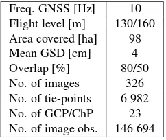
permanent markers. The block consists of 12 parallel lines and 4 lines perpendicular to them, flown in two separate flight heights. The data is characterised in Tab. 2. The maximal separation be-tween the MAV and base station was 500 m. The block configu-ration is depicted in Fig. 3. The ground accuracy was evaluated at independent ChPs.
Freq. GNSS [Hz] 10 Flight level [m] 130/160 Area covered [ha] 98
Mean GSD [cm] 4
Overlap [%] 80/50
No. of images 326 No. of tie-points 6 982 No. of GCP/ChP 23 No. of image obs. 146 694
Table 2. Summary of aquired data.
3. IN-FLIGHT TRAJECTORY PRECISION
The GNSS data from both receivers was processed in GrafNav (Novatel, 2016) and interpolated for each camera event. While the reference trajectory has ambiguity fixed throughout the entire flight, the NEO-8T data allows only a float solution. Neverthe-less, as long as the float ambiguities converge to a stable value, the float solution may be considered as accurate enough, espe-cially in a relative aerial control.
Figure 3. 3D view on the scene with camera stations, GCPs and a point cloud of tie-points from Pix4Dmapper Pro.
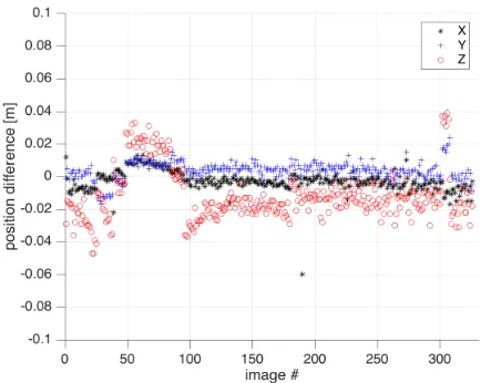
The two sets of camera position parameters derived from tested vs. reference data are compared in Fig. 4 in an absolute, and in Fig. 5 in a relative way, i.e. differences between two positions of two consecutive camera stations. It can be seen that rather small (<10 cm) differences/drift in absolute positions are eliminated by differencing.
Figure 5. Differences in relative camera positions between high-end and low-cost L1 only (ambig. float) GNSS receivers.
4. MAPPING ACCURACY
4.1 Absolute Aerial Control
As a next step, Pix4Dmapper Pro (Pix4D SA, 2016) was used to obtain image observations and initial attitude parameters. The re-constructed scene can be seen in Fig. 3. Bundle adjustment was carried out in TopoBun (Rehak and Skaloud, 2016) and Pix4D mapper Pro without GCPs and with self-calibrated interior ori-entation (IO) parameters (c, x0, y0, K1, K2) in the following configurations:
I. Processing with a known lever-arm. The calibrated offset has the value of a(ax, ay, az) = [−433, −31, 147] mm. This value is a calibrated lever-arm from a ground cali-bration based on the pseudo-measurement technique (Ellum and El-Sheimy, 2002). This lever-arm is introduced in the adjustment as a weighted observation withσax,y = 1.5cm andσaz = 2cm.
II. Processing without a priori knowledge of the lever-arm, i.e. the initial offset is zero, its incertitudeσax, ay, az = 0.5m,
and is estimated in BA as an additional parameter.
III. The lever-arm is not considered, i.e. it is assumed that there is no offset in camera positions.
The results of the cases I-III are summarised in Tab. 3. In general, the projects processed with camera position parameters from the
Javad receiver manifest better ground accuracy in overall. In the case the lever-arm is known, the achieved accuracy is close to 1 pixel in position and height for the Javad, and 1.5-2 pixels for the U-Blox considering the average GSD of 4 cm.
The processing II demonstrated the ability of the BA to resolve initially unknown lever-arm, but not better than 5 cm along cam-era’s x-axis. Indeed, this could be a typical mapping scenario for consumer drones to which a GNSS receiver is added, and a lever-arm between a camera and an antenna is not known. The differences between the processing I and II are significant mainly in X and Z coordinates. This is due to the unconstrained lever-arm. The system is over-parametrised and estimated parameters are highly correlated, particularly theZ0−c−azandx0−ax. As expected, the lever-arm is highly correlated with IO param-eters and camera positions, as shown in their variations in Tab. 3. There is a significant change of thex0 coordinate between processing I and III, i.e. with and without the lever-arm. The missing lever-arm offset is absorbed by estimated values of the principal point and camera constant, but it is not projected to the ground shift in the Z coordinate as it happened in the case II. Some pertinent correlation parameters are stated in Tab. 4. These are calculated during the BA project of the type II with positions from the Javad receiver.
In general, the Javad receiver provided higher accuracy of abso-lute positions. The resulting accuracy measured at independent ChPs lies in the case I in the level of∼ 1pixel in position and height, respectively. The U-Blox receiver can deliver accuracy in the level of∼2pixels in position and∼1.5pixels in height without the support of GCPs. Due to the size of the lever-arm, i.e. theaxoffset is significantly larger thanaz, the horizontal ground accuracy is more influenced than its vertical component.
Parameters Correlation [0-100%]
X0−ax 35
Y0−ay 36
Z0−az 79
Z0−c 62
x0−ax 68
y0−ay 84
c−az 79
Table 4. Significant correlations of a randomly selected image between the lever-arm (ax,y,z), projection centre (X0, Y0, Y0), principal point (x0, y0), and camera constantc.
4.2 Relative Aerial Control
Relative observations were calculated from both sets of camera absolute positions. In order to orient the network, at least one GCP must be added. In practice, this can be, e.g. the base station
Test
Accuracy IO
[mm]
Lever-arm [mm]
Rx Mean ChP [mm] RMS ChP [mm]
X Y Z X Y Z c x0 y0 ax ay az
Javad
I. TPB: known lever-arm -1 14 31 42 27 49 15.8315 -0.0069 0.0187 -479 -19 142
II. TPB: unknown lever-arm -1 14 93 41 27 100 15.8351 -0.0027 0.0181 -528 -1 59
III. TPB: no lever-arm -1 15 107 46 36 115 15.8386 -0.0635 0.0167 - -
-Pix4D: no lever-arm 0 -19 -75 43 35 90 15.8421 0.0382 0.0180 - -
-U-Blox
I. TPB: known lever-arm 46 34 -16 64 42 46 15.8376 -0.0050 0.0191 -487 -19 123
II. TPB: unknown lever-arm 46 34 193 63 42 188 15.8491 0.0002 0.0200 -535 -30 -174
III. TPB: no lever-arm 47 35 47 67 47 63 15.8440 -0.0626 0.0171 - -
-Pix4D: no lever-arm -47 -37 -34 64 47 63 15.8452 0.0373 0.0175 - -
Test
Accuracy IO
[mm]
Rx Mean ChP [mm] RMS ChP [mm]
X Y Z X Y Z c x0 y0
Javad I. TPB: 1 GCP, known lever-arm 28 4 -26 59 28 62 15.8372 -0.0063 0.0179
I. TPB: 4 GCPs, known lever-arm -25 -9 -8 51 36 49 15.8370 -0.0064 0.0180
U-Blox I. TPB: 1 GCP, known lever-arm 28 3 -31 59 27 64 15.8390 -0.0059 0.0182
I. TPB: 4 GCPs, known lever-arm -25 -8 -6 51 35 49 15.8388 -0.0059 0.0182
Table 5. Mapping accuracy at 22 ChPs, with 1 or 4 GCPs, and with relative aerial position control.
point provided it is visible in the imagery. Thus, two scenarios are considered. Relative aerial observations with one or four, well-distributed GCPs. The processing was performed for the case I due to the assumption that a lever-arm cannot be determined well with relative position control unless the flying speed varies signif-icantly, which was not the case. Therefore, the camera absolute positions were first corrected for the lever-arm and then differen-tiated between two consecutive epochstiandtjfordttj<10s, according to Eq. 2. The camera attitude values for applying lever-arm corrections were taken from BA using absolute aerial position control (within Pix4Dmapper Pro project). On the con-trary, MAV platforms with short lever-arms between a camera and a GNSS antenna, such as the eBee (senseFly, 2015), can use attitude from the autopilot’s IMU (Inertial Measurement Unit). For that, the autopilot’s internal clock must be time-synchronised with the GNSS receiver and the camera.
The results from four adjustment projects are summarised in Tab. 5. When the relative observations of camera perspective centres replace the absolute ones and one GCP is used, the ground accu-racy lies in the level of∼ 1.5pixels in horizontal position and height. After adding 3 additional GCPs for the total of 4, the ac-curacy improved only marginally in height component by∼1.5 cm to∼1pixel.
4.3 Feasibility of L1 KAR
Although Kinematic Ambiguity Resolution (KAR) with single-frequency phase observations is possible, the reliability of the obtained solution is rather low as it depends not only on the qual-ity of the obtained signal, but it requires relatively long tracking continuity without cycle slips. For this reason, a float ambigu-ity solution was considered for the low-cost receiver. Indeed, the convergence of float ambiguities over the time period of 5 to 10 minutes is a good indicator that L1-only KAR may be achieved over a shorter time period. The needed time span is typically 3-5 times longer than with multi-frequency data. Considering a du-ration of a flight-line of 60-120 s, we have chosen a minimum of 1.5 minutes of continuous data for the KAR. This resulted in fixed aerial positions that were compared to the reference. This com-parison is depicted in Fig. 6 for all used photos. The RMS of dis-crepancies is<1cm horizontally and<2cm vertically. As the empirically verified noise-level of the multi-frequency position-ing for the employed MAV is around2cm (Rehak and Skaloud, 2015), such differences can be considered insignificant.
These results seem encouraging, yet cannot be generalised for all platforms and conditions. The requirement on longer con-tinuity of phase data without cycle-slips is problematic under higher dynamics. Shorter observation spans lead to lower reli-ability of L1 KAR and thus possibly biased-position determina-tion due to wrong ambiguities. As long as such bias is constant between subsequent photos (i.e. several seconds), it can be effec-tively mitigated by employing relative aerial control as investi-gated in (Skaloud and Lichti, 2014), (Rehak and Skaloud, 2015), and herein.
Figure 6. Differences in absolute camera positions between high-end and low-cost L1 only (ambig.-fixed) GNSS receivers.
5. CONCLUSIONS AND PERSPECTIVES
This contribution demonstrated the potential of a low-cost GNSS receiver to deliver absolute and relative aerial observations. These observations were used in mapping configurations with and with-out GCPs, respectively. The results were evaluated with respect to ChPs accuracy, and by assessing precision values of calibrated parameters. It was shown that cm-level ground accuracy is achiev-able without GCPs with absolute and relative aerial observations derived from a low-cost receiver. An integration of such a re-ceiver on a MAV platform is not trivial due to its higher sen-sitivity to vibrations, electromagnetic interference, and limited synchronisation possibilities. Also, the quality and/or continuity of the phase data observations on such receivers can be rapidly decreased by higher dynamics that can occur due to air turbu-lence, or platform’s control manoeuvres. Despite that, it was empirically demonstrated that the successful L1 KAR provides practically the same precision as that of the high-end receiver. Whenever the reliability of L1 KAR is insufficient, the method of relative aerial position control provides an effective protection against positioning bias. Nevertheless, as low-cost dual (or triple) frequency receiver boards are expected to become a standard part of commercial drones in the future, the budget vs. performance ratio may lose its significance.
REFERENCES
Aibotix GmbH, Part of Hexagon, 2016. Aibotix X6 UAV.
https://www.aibotix.com/en/. [Online; accessed 13-August-2016].
Benoit, L., Martin, O. and Thom, C., 2015. Low-cost GPS Sensors for deformation monitoring. GIM International29(4), pp. 25–27.
Colomina, I., 2007. From off-line to on-line geocoding: the evo-lution of sensor orientation. In: D. Fritsch (ed.), Photogrammet-ric Week, Stuttgart, Germany, pp. 173–183.
CSG Shop, 2016. UBLOX NEO-M8T.http://www.csgshop. com/product.php?id_product=205. [Online; accessed 26-October-2016].
Eling, C., Klingbeil, L., Wieland, M. and Kuhlmann, H., 2014. Direct georeferencing of micro-aerial vehicles - system design, system calibration and first evaluation tests. Journal of pho-togrammetry, remote sensing and geoinformation processing (PFG)4, pp. 227–237.
Ellum, C. and El-Sheimy, N., 2002. Inexpensive Kinematic Attitude Determination from MEMS-Based Accelerometers and GPS-Derived Accelerations. NAVIGATION: Journal of The In-stitute of Navigation49(3), pp. 117–126.
Gerke, M. and Przybilla, H.-J., 2016. Accuracy Analysis of Pho-togrammetric UAV Image Blocks: Influence of Onboard RTK-GNSS and Cross Flight Patterns. Photogrammetrie, Fernerkun-dung, Geoinformation (PFG)2016(1), pp. 17–30.
Javad GNSS Inc., 2016. Javad TRE-G3T.http://www.javad. com/jgnss/products/oem/. [Online; accessed 14-August-2016].
Li, K. and Stueckmann-Petring, J., 1992. Methods and results of combined adjustment utilizing kinematic GPS positioning and photogrammetric data. 29, pp. 213–213.
MAVinci GmbH, 2015. Sirius Pro.http://www.mavinci.com. [Online; accessed 13-August-2016].
Maxtena, 2016. Rugged L1/L2 GPS GLONASS Active Antenna. http://www.maxtena.com/products/helicore/ m1227hct-a2-sma/?v=1ee0bf89c5d1. [Online; accessed 31-October-2016].
Meier, L., Tanskanen, P., Heng, L., Lee, G., Fraundorfer, F. and Pollefeys, M., 2012. PIXHAWK: A micro aerial vehicle de-sign for autonomous flight using onboard computer vision. Au-tonomous Robots33(1-2), pp. 21–39.
Mongredien, C., Hide, C., Faihust, P. and Ammann, D., 2016. Centimeter positioning for UAVs and mass-market applications. GPS World.
Novatel, 2016. Waypoint Software. http://www.novatel. com/products/software/. [Online; accessed 31-October-2016].
Odolinski, R. and Teunissen, P., 2016. Single-frequency, dual-gnss versus dual-frequency, single-dual-gnss: a low-cost and high-grade receivers gps-bds rtk analysis. Journal of Geodesy90, pp. 1255–1278.
Pix4D SA, 2016. Pix4Dmapper Pro 3.0. http://pix4d.com/. [Online; accessed 15-November-2016].
Rehak, M. and Skaloud, J., 2015. Fixed-wing micro aerial vehi-cle for accurate corridor mapping. In:ISPRS Annals of the Pho-togrammetry, Remote Sensing and Spatial Information Sciences, Vol. II-1/W4, Toronto, Canada, pp. 23–31.
Rehak, M. and Skaloud, J., 2016. Applicability of new ap-proaches of sensor orientation to micro aerial vehicles. In:ISPRS - Annals of the Photogrammetry, Remote Sensing and Spatial In-formation Sciences, Vol. III-3, Prague, Czech Republic, pp. 441– 447.
Rehak, M., Skaloud, J. and Mabillard, R., 2013. A micro-uav with the capability of direct georeferencing. In:UAV-g, Rostock, Germany.
senseFly, 2015. senseFly drones and cameras. http://www. sensefly.com. [Online; accessed 13-August-2016].
Skaloud, J. Rehak, M. and Lichti, D., 2014. Mapping with MAV: Experimental study on the contribution of absolute and relative position control. In: ISPRS-The International Archives of the Photogrammetry Remote Sensing and Spatial Information Sci-ences, Vol. 40-3/W1, Castelldefels, Spain, pp. 123–129.
Sony, 2016. Sony NEX-5R. http://www.sony.co.uk/ support/en/product/nex-5r. [Online; accessed 14-August-2016].
Stempfhuber, W. and Buchholz, M., 2011. A precise, low-cost RTK GNSS system for UAV applications. In:ISPRS - The Inter-national Archives of the Photogrammetry, Remote Sensing and Spatial Information Sciences, Zurich, Switzerland, pp. 289–293.
Survey Group, 2015. Taming a monster – large-scale RTK corridor mapping in remotest Australia.
https://www.sensefly.com/fileadmin/user_ upload/sensefly/images/web2014/applications/ senseFly-Case-Study-eBee-RTK-Talawana.pdf. [Online; accessed 12-September-2016].