KEY WORDS:Classification, Segmentation, Regularization, LiDAR, Urban, Point Cloud, Random Forest
ABSTRACT:
We consider the problem of the semantic classification of 3D LiDAR point clouds obtained from urban scenes when the training set is limited. We propose a non-parametric segmentation model for urban scenes composed of anthropic objects of simple shapes, partionning the scene into geometrically-homogeneous segments which size is determined by the local complexity. This segmentation can be integrated into a conditional random field classifier (CRF) in order to capture the high-level structure of the scene. For each cluster, this allows us to aggregate the noisy predictions of a weakly-supervised classifier to produce a higher confidence data term. We demonstrate the improvement provided by our method over two publicly-available large-scale data sets.
INTRODUCTION
Automatic interpretation of large 3D point clouds acquired from terrestrial and mobile LiDAR scanning systems has become an important topic in the remote sensing community (Munoz et al., 2009; Weinmann et al., 2015), yet it presents numerous techni-cal challenges. Indeed, the high volume of data and the irregular structure of LiDAR point clouds make assigning a semantic label to each point a difficult endeavor. Furthermore the production of a precise ground truth is particularly difficult and time-consuming. However, LiDAR scans of urban scenes display some form of regularity and a specific structure can then be exploited to im-prove the accuracy of a noisy semantic labeling.
Foremost, the high precision of LiDAR acquisition methods im-plies that the number of points far exceeds the number of objects in a scene. Consequently, the sought semantic labeling can be expected to display high spatial regularity. Although the method presented in (Weinmann et al., 2015) relies on the computation of local neighborhood, the resulting classification is not regular in general, as observed in Figure 1b. This regularity prior has been incorporated into context-based graphical models (Anguelov et al., 2005; Shapovalov et al., 2010; Niemeyer et al., 2014) and a structured regularization framework (Landrieu et al., 2017a), significantly increasing the accuracy of input pointwise classifi-cations.
Pre-segmentations of the point cloud have been used to model long-range interactions and to decrease the computational burden of the regularization. The segments obtained can then be incor-porated into multi-scale graphical models to ensure a spatially-regular classification. However, the existing models require set-ting the parameters of the segments in advance, such as their max-imum radius (Niemeyer et al., 2016; Golovinskiy et al., 2009), the maximum number of points in each segment (Lim and Suter, 2009), or the total number of segment (Shapovalov et al., 2010).
The aim of our work is to leverage the underlying structure of the point cloud to improve a weak classification obtained from very few annotated points, with a segmentation that requires no preset size parameters. We observe that the structure of urban scenes
is mostly shaped by man-made objects (roads, façades, cars...), which are geometrically simple in general. Consequently, well-chosen geometric features associated to their respective points can be expected to be spatially regular. However the extent and number of points of the segments can vary a lot depending on the nature of the corresponding objects. We propose a formulation of the segmentation as a structured optimization problem in order to retrieve geometrically simple super-voxels. Unlike other preseg-mentation approaches, our method allows the segments’ size to be adapted to the complexity of the local geometry, as illustrated in Figure 1c.
Following the machine-learning principle that an ensemble of weak classifiers can perform better than a strong one (Opitz and Maclin, 1999), a consensus prediction is obtained from the seg-mentation by aggregating over each segment the noisy predic-tions of its points obtained from a weakly-supervised classifier. The structure induced by the segmentation and the consensus pre-diction can be combined into a conditional random field formu-lation to directly classify the segments, and reach state-of-the-art performance from a very small number of hand-annotated points.
Related Work
Point-wise classification:Weinmann et al. (2015) propose a clas-sification framework based on 3D geometric features which are derived from local neighborhood of optimal size.
Context-based graphical models:the spatial regularity of a se-mantic labeling can be enforced by graphical models such as ran-dom Markov fields (Anguelov et al., 2005; Shapovalov et al., 2010), and its discriminative counterpart, the conditional random field (Niemeyer et al., 2014; Landrieu et al., 2017b). The unary terms are computed by a point-wise classification with a random forest classifier, while the pairwise terms encode the probability of transition between the semantic classes.
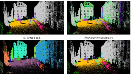
(a) Ground truth (b) Pointwise classification
(c) Geometrically homogeneous segmentation (d) Segmentation-aided regularization
Figure 1. Illustration of the different steps of our method: the pointwise, irregular classification 1b is combined with the geometrically homogeneous segmentation 1c to obtain a smooth, objects-aware classification 1d. In Figures 1a, 1b , 1d, the semantic classes are represented with the following color code:vegetation,façades,hardscape,acquisition artifacts,cars,roads. In Figure 1c, each segment is represented by a random color.
method based on a predefined number of points in each pixel, and a color homogeneity prior. In Niemeyer et al. (2016), the segments are determined using a prior pointwise-classification. A multi-tier CRF is then constructed containing both points and voxels nodes. An iterative scheme is then performed, which alter-nates between inference in the multi-tier CRF and the computa-tion of the semantically homogeneous segments with a maximum radius constraint. In Shapovalov et al. (2010) the presegmenta-tion is obtained through the k-means algorithm, which requires defining the number of clusters in the scene in advance. Fur-thermore k-means produces isotropic clusters whose size doesn’t adapt to the geometrical complexity of the scene. In Dohan et al. (2015), a hierarchical segmentation is computed using the fore-ground/background segmentation of Golovinskiy et al. (2009), which uses a preset horizontal and vertical radius as parameters. The segments are then hierarchically merged then classified.
Problem formulation
We consider a 3D point cloudV corresponding to a LiDAR ac-quisition in an urban scene. Our objective is to obtain a classifica-tion of the points inV between a finite set of semantic classesK. We consider that we only have a small number of hand-annotated points as a ground truth from a similar urban scene. This number must be small enough that it can be produced by an operator in a reasonable time, i.e. no more than a few dozen per class.
We present the consituent elements of our approach in this sec-tion, in the order in which they are called.
Feature and graph computation: For each point, we com-pute a vector of geometrical features, described in Section 2.1. In Section 2.3 we present how the adjacency relationship between points is encoded into a weighted graph.
Segmentation in geometrically homogeneous segments: The segmentation problem is formulated as a structured optimization problem presented in Section 3.1, and whose solution can be ap-proximated by a greedy algorithm. In section 3.2, we describe how the higher-level structure of the scene can be captured by a graph obtained from the segmentation.
Contextual classification of the segments: In Section 4, we present a CRF which derived its structure from the segmentation, and its unary parameter from the aggregation of the noisy pre-diction of a weakly supervised classifier. Finally, we associate the label of the corresponding segment to each point in the point cloud.
FEATURES AND GRAPH COMPUTATION In this section, we present the descriptors chosen to represent the local geometry of the points, and the adjacency graph capturing the spatial structure of the point cloud.
With a view that the training set is small, and to keep the compu-tational burden of the segmentation to a minimum, we voluntarily limit the number of descriptors used in our pointwise classifica-tion. We insist on the fact that the segmentation and the classifi-cation do not necessarily use the same descriptors.
Local descriptors
In order to describe the local geometry of each point we define four descriptors: linearity, planarity, scattering and verticality, which we represent in Figure 4.
us to qualify the shape of the local neighborhood by deriving the
The linearity describes howelongatedthe neighborhood is, while the planarity assesses how well it is fitted by a plane. Finally, high-scattering values correspond to an isotropic and spherical neighborhood. The combination of these three features is called dimensionality.
In our experiments, the vertical extent of the optimal neighbor-hood proved crucial for discriminating roads and façades, and between poles and electric wires, as they share similar dimension-ality. To discriminate this class, we introduce a novel descriptor calledverticalityalso obtained from the eigen vectors and values defined above. Letu1, u2, u3be the three eigenvectors associ-ated withλ1, λ2, λ3 respectively. We define the unary vector of principal direction inR3+as the sum of the absolute values of the coordinate of the eigenvectors weighted by their eigenvalues:
[ˆu]i∝ 3 X
j=1
λj|[uj]i|, pouri= 1,2,3 et kuˆk= 1
We argue that the vertical component of this vector characterizes the verticality of the neighborhood of a point. Indeed it reaches its minimum (equal to zero) for an horizontal neighborhood, and its maximum (equal to 1) for a linear vertical neighborhood. A vertical planar neighborhood, such as a façade, will have an inter-mediary value (around 0.7). This behavior is illustrated at Figure in Figure 4.
To illustrate the weak number of features selected, we represent their respective value and range in Figure 2.
Non-local descriptors
Although the neighborhoods’ shape of 3D points determine their local geometry, and allows us to compute a geometrically homo-geneous segmentation, this not sufficient for classification. Con-sequently, we use two descriptors of the global position of points: elevation and position with respect to the road.
Computing those descriptors first requires determining the extent of the road with high precision. A binary road/non-road classifi-cation is performed using only the local geometry descriptors and a random forest classifier, which achieves very high accuracy and a F-score over 99.5%. From this classification a simple elevation model is computed, allowing us to associate a normalized height with respect to the road to each 3D point.
linearity planarity scattering verticality 0
0.2
Figure 2. Means and standard deviations of the local descriptors in the Oakland dataset for the following classes: wires, poles,
façades,roads,vegetation.
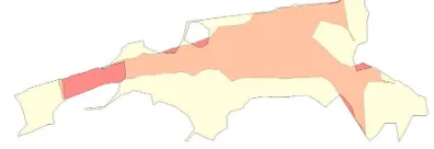
Figure 3. α-shape of the road on our Semantic3D example. In red, the horizontal extent of the road; in yellow, the extent of the non-road class.
To estimate the position with respect to the road we compute the two-dimensionalα-shape (Akkiraju et al., 1995) of the points of the road projected on the zero elevation level, as represented in Figure 3. This allows us to compute theposition with respect to the roaddescriptor, equal to1if a point is outside the extent of the road,0.5if the point is close to the edge of theα-shape with a tolerance of1m, and0otherwise.
Adjacency graph
The spatial structure of a point cloud can be represented by an unoriented graphG= (V, E), in which the nodes represent the points of the cloud, and the edges encode theiradjacency rela-tionship. We compute the10-nearest neighbors graph, as advo-cated in (Niemeyer et al., 2011). Remark that this graph defines a symmetric graph-adjacency relationship which isdifferentfrom the optimal neighborhood used in Section 2.1.
SEGMENTATION INTO HOMOGENEOUS SEGMENTS Potts energy segmentation
To each point, we associate its local geometric feature vector
fi ∈ R4(dimensionality and verticality), and compute a piece-wise constant approximationg⋆
of the signalf ∈RV×4 struc-tured by the graphG.g⋆is defined as the vector ofRV×4 mini-mizing the followingPotts segmentation energy:
(a) Dimensionality (b) Verticality
(c) Elevation (d) Position with respect to the road
Figure 4. Representation of the four local geometric descriptors as well as the two global descriptors. In (a), the dimensionality vector [linearity, planarity, scattering] is color-coded by a proportional [red, green, blue] vector. In (b), the value of the verticality is represented with a color map going from blue (low verticality - roads) to green/yellow (average verticality - roofs and façades) to red (high verticality - poles). In (c), is represented the elevation with respect to the road. In (d), the position with respect to the road is represented with the following color-code: inside the roadα-shape in red, bordering in green, and outside in blue.
withδ(· 6= 0) the function ofR4 :7→ {0,1}equal to0in 0 and1everywhere else. The first part of this energy is the fidelity function, ensuring that the constant components ofg⋆
correspond to homogeneous values off. The second part is the regularizer which adds a penalty for each edge linking two components with different values. This penalty enforces the simplicity of the shape of the segments. Finallyρis the regularization strength, deter-mining the trade off between fidelity and simplicity, and implic-itly determining the number of clusters.
This structured optimization problem can be efficiently approxi-mated with the greedy graph-cut basedℓ0-cut pursuit algorithm presented in Landrieu and Obozinski (2016). The segments are defined as the constant connected components of the piecewise constant signal obtained.
The benefit of this formulation is that it does not require defining a maximum size for the segments in terms of extent or points. Indeed large segments of similar points, such as roads or façades, can be retrieved. On the other hand, the granularity of the seg-ments will increase where the geometry gets more complex, as illustrated in Figure 1c.
For the remainder of the article we denoteS = (S1,· · ·, Sk) the non-overlapping segmentation ofV obtained when approxi-mately solving the optimization problem.
Segment-graph
We argue that since the segments capture the objects in the scene, the segmentation represents its underlying high-level structure. To obtain the relationship between objects, we build the segment-graph, which is defined asG = (S,E, w)in which the segments ofSare the nodes ofG. Erepresents the adjacency relationship
Figure 5. Adjacency structure of the segment-graph. The edges between points are represented in black , the segmentation and the adjacency of its components in blue: .
between segments, whilewencodes the weight of their boundary, as represented in Figure 5. We define two segments as adjacent if there is an edge inElinking them, andwas the total weight of the edges linking those segments:
(
E ={(s, t)∈S2 | ∃(i, j)∈E∩(s×t)}
ws,t =|E∩(s×t)|, ∀(s, t)∈S2.
CONTEXTUAL CLASSIFICATION OF THE SEGMENTS
To enforce spatial regularity, Niemeyer et al. (2014) defines the optimal labelingl⋆ of a point cloud as maximizing the poste-rior distributionp(l | f′
)in a conditional random field model structured by an adjacency graphG, withf′
the probability of nodei being in statek, andM(i,j),(k,l) = log(p(li = k, lj = l | fi′, f
′
j))the entrywise logarithm of the probability of observing the transition(k, l)at(i, j).
As advocated in Niemeyer et al. (2014), we can estimatep(li =
k | f′
i) with a random forest probabilistic classifier pRF. To
avoid infinite values, the probabilitypRF is smoothed by taking
a linear interpolation with the constant probability:p(k|fi) = (1−α)pRF(k|f′i)+α/|K|withα= 0.01and|K|the cardinal-ity of the class set. The authors also advocate learning the transi-tion probability from the difference of the features vectors. How-ever, our weak supervision hypothesis prevents us from learning the transitions, as it would require annotations covering the|K|2 possible combinations extensively. Furthermore the annotation would have to be very precise along the transitions, which are of-ten hard to distinguish in point clouds. We make the simplifying hypothesis thatM is of the following form :
M(i,j),(k,l)= (
0 ifk=l
σ else, (2)
withσa non-negative value, which can be determined by cross-validation.
Leveraging the hypothesis that the segments obtained in in Sec-tion 3.1 correspond to semantically homogeneous objects, we can assume that the optimal labeling will be constant over each seg-ment ofS. In that regard, we propose a formulation of a CRF structured by the segment-graphGto capture the organization of the segments. We denoteL⋆
the labeling ofSdefined as:
L⋆= arg max probability of segmentsbeing in statek multiplied by the car-dinality of s. We define this probability as the average of the probability of each point contained in the segment:
p(Ls=k| {f
Note that the influence of the data term of a segment is deter-mined by its cardinality, since the classification of the points re-mains the final objective. Likewise, the cost of a transition be-tween two segments is weighted by the total weight of the edges at their interfacews,t, and represents the magnitude of the inter-action between those two segments.
Following the conclusions of Landrieu et al. (2017b), we ap-proximate the labelling maximizing the log-likelihood with the maximum-a-priori principle using theα-expansion algorithm of Boykov et al. (2001), with the implementation of Schmidt (2007).
It is important to remark that the segment-based CRF only in-volves the segment-graphG, which can be expected to be much
Data
To validate our approach, we consider two publicly available data sets.
We first consider the urban part of the Oakland benchmark intro-duced in Munoz et al. (2009), comprised of 655.297 points ac-quired by mobile LiDAR. Some classes have been removed from the acquisition (i.e. cars or pedestrians) so that there are only 5 left: electric wires, poles/trunks, façcades, roads and vegetation. We choose to exclude the tree-rich half of the set as the segmen-tation results are not yet satifying at the trunk-tree interface.
We also consider one of the urban scenes in the Semantic3D benchmark1, downsampled to 3.5 millions points for memory reasons. This scene, acquired with a fixed LiDAR, contains 6 classes : road, façade, vegetation, car, acquisition artifacts and hardscape.
For each class we hand-pick a small number of representative points such that the discriminative nature of our features illus-trated in Figure 2 is represented. We select 15 points per classes for Oakland and 25 to 35 points for semantic3D, for respective totals of 75 and 180 points.
Metric
To take into account the imbalanced distribution of each class (roads and façades comprise up to 80% of the points), we use the unweighted average of the F-scores to evaluate the classifica-tion results. Consequently, a classificaclassifica-tion with decent accuracy over all classes will have a higher score than a method with high accuracy over some classes but poor results for others.
Competing methods
To compare the efficiency of our implementation to the state-of-the-art we have implemented the following methods:
• Pointwise:we implemented the pointwise classification re-lying on optimal neighborhoods of Weinmann et al. (2015), with a random forest (Breiman, 2001) and restricted our-selves to the six geometric features presented in Section 2.1.
• CRF regularization: we implemented the CRF defined in (1) without aid from the segmentation.
Results
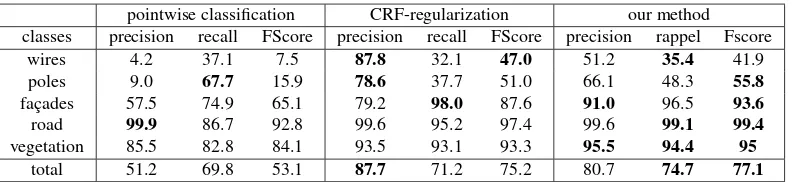
In Tables 1 and 2, we represent the classification results of our method and the competing methods for both datasets. We ob-serve that both the CRF and the presegmentation approach sig-nificantly improve the results compared to the point-wise classi-fication. Although the improvement in term of global accuracy
pointwise classification CRF-regularization our method classes precision recall FScore precision recall FScore precision rappel Fscore
wires 4.2 37.1 7.5 87.8 32.1 47.0 51.2 35.4 41.9
poles 9.0 67.7 15.9 78.6 37.7 51.0 66.1 48.3 55.8
façades 57.5 74.9 65.1 79.2 98.0 87.6 91.0 96.5 93.6
road 99.9 86.7 92.8 99.6 95.2 97.4 99.6 99.1 99.4
vegetation 85.5 82.8 84.1 93.5 93.1 93.3 95.5 94.4 95
total 51.2 69.8 53.1 87.7 71.2 75.2 80.7 74.7 77.1
Table 1. Precision, recall and FScore in % for the Oakland benchmark. The global accuracy are respectively 85.2%, 94.8% et 97.3%. In bold, we represent the best value in each category.
pointwise classification CRF-regularization our method classes precision recall FScore precision recall FScore precision rappel Fscore
road 98.7 96.8 97.7 97.6 99.0 98.3 97.5 98.7 98.1
vegetation 14.2 82.9 24.2 49.7 84.7 62.6 52.1 93.7 67.0
façade 99.6 88.1 93.5 99.5 97.9 98.7 99.7 98.2 98.8
hardscape 74.2 71.4 73.1 93.7 88.7 91.2 92.7 90.4 91.5
artifacts 18.3 37.5 24.6 77.9 42.1 54.7 73.8 39.3 51.3
cars 28.6 54.8 37.6 66.5 86.2 75.1 84.0 90.0 82.3
total 55.7 71.9 58.4 80.8 83.1 80.1 83.3 85.0 82.3
Table 2. Precision, recall and FScore in % for the Semantic3D benchmark. The global accuracy are respectively 88.4%, 96.9% et 97.2%. In bold, we represent the best value in each category.
of our method compared to the CRF-regularization is limited (a few % at best), the quality of the classification is improved signif-icantly for some hard-to-retrieve classes such as poles, wires, and cars. Furthermore, our method provides us with a object-level segmentation as well.
CONCLUSION
In this article, we presented a classification process aided by a ge-ometric pre-segmentation capturing the high-level organization of an urban scene. We showed that this segmentation allowed us to formulate a CRF to directly classify the segments, improv-ing the results over the CRF-regularization Further developments should focus on improving the quality of the segmentation near loose and scattered acquisition such as foliage. Another possible improvement would be to better exploit the context of the tran-sition. Indeed the form of the transition matrix in (2) is too re-strictive, as it does not take into account rules such as "the road is below the façcade" or the "tree-trunk is more likely than foliage-road". Although the weakly-supervised context excludes learning the transition, it would nonetheless be beneficial to incorporate the expertise of the operator.
References
Akkiraju, N., Edelsbrunner, H., Facello, M., Fu, P., Mücke, E. and Varela, C., 1995. Alpha shapes: definition and software. In:Proceedings of the 1st International Computational Geom-etry Software Workshop, Vol. 63, p. 66.
Anguelov, D., Taskarf, B., Chatalbashev, V., Koller, D., Gupta, D., Heitz, G. and Ng, A., 2005. Discriminative learning of markov random fields for segmentation of 3d scan data. In: 2005 IEEE Computer Society Conference on Computer Vision and Pattern Recognition (CVPR’05), Vol. 2, IEEE, pp. 169– 176.
Boykov, Y., Veksler, O. and Zabih, R., 2001. Fast approximate energy minimization via graph cuts. IEEE Transactions on
Pattern Analysis and Machine Intelligence23 (11), pp. 1222– 1239.
Breiman, L., 2001. Random forests. Machine learning45(1), pp. 5–32.
Demantké, J., Mallet, C., David, N. and Vallet, B., 2011. Dimen-sionality based scale selection in 3d lidar point clouds. The International Archives of the Photogrammetry, Remote Sens-ing and Spatial Information Sciences38(Part 5), pp. W12.
Dohan, D., Matejek, B. and Funkhouser, T., 2015. Learning hi-erarchical semantic segmentations of lidar data. In:3D Vision (3DV), 2015 International Conference on, IEEE, pp. 273–281.
Golovinskiy, A., Kim, V. G. and Funkhouser, T., 2009. Shape-based recognition of 3d point clouds in urban environments. In: Computer Vision, 2009 IEEE 12th International Confer-ence on, IEEE, pp. 2154–2161.
Landrieu, L. and Obozinski, G., 2016. Cut pursuit: fast al-gorithms to learn piecewise constant functions on general weighted graphs.
Landrieu, L., Raguet, H., Vallet, B., Mallet, C. and Weinmann, M., 2017a. A structured regularization framework for spatially smoothing semantic labelings of 3d point clouds.
Landrieu, L., Weinmann, M. and Mallet, C., 2017b. Comparison of belief propagation and graph-cut approaches for contextual classification of 3d lidar point cloud data.
Lim, E. H. and Suter, D., 2009. 3d terrestrial lidar classifications with super-voxels and multi-scale conditional random fields. Computer-Aided Design41(10), pp. 701–710.
Prague, Czech Republic, Göttingen: Copernicus GmbH.
Niemeyer, J., Wegner, J. D., Mallet, C., Rottensteiner, F. and So-ergel, U., 2011. Conditional random fields for urban scene classification with full waveform lidar data. In: Photogram-metric Image Analysis, Springer, pp. 233–244.
Opitz, D. and Maclin, R., 1999. Popular ensemble methods: An empirical study.Journal of Artificial Intelligence Research11, pp. 169–198.
Schmidt, M., 2007. A Matlab toolbox for probabilistic undirected graphical models. http://www.cs.ubc.ca/~schmidtm/ Software/UGM.html.
Shapovalov, R., Velizhev, E. and Barinova, O., 2010. Non-associative markov networks for 3d point cloud classification. In: International Archives of the Photogrammetry, Remote Sensing and Spatial Information Sciences XXXVIII, Part 3A, Citeseer.