SCALE INVARIANT FEATURE TRANSFORM PLUS HUE FEATURE
Mohammad B.Daneshvara
aDaneshvar innovation group, Signal processing department, 4763843545 Qaem Shahr, Iran, [email protected]
KEY WORDS: Euclidean distance, Keypoint, Hue feature, Feature extraction, Mean square error, Image matching.
ABSTRACT:
This paper presents an enhanced method for extracting invariant features from images based on Scale Invariant Feature Transform (SIFT). Although SIFT features are invariant to image scale and rotation, additive noise, and changes in illumination but we think this algorithm suffers from excess keypoints. Besides, by adding the hue feature, which is extracted from combination of hue and illumination values in HSI colour space version of the target image, the proposed algorithm can speed up the matching phase. Therefore, we proposed the Scale Invariant Feature Transform plus Hue (SIFTH) that can remove the excess keypoints based on their Euclidean distances and adding hue to feature vector to speed up the matching process which is the aim of feature extraction. In this paper we use the difference of hue features and the Mean Square Error MSE of orientation histograms to find the most similar keypoint to the under processing keypoint. The keypoint matching method can identify correct keypoint among clutter and occlusion robustly while achieving real-time performance and it will result a similarity factor of two keypoints. Moreover removing excess keypoint by SIFTH algorithm helps the matching algorithm to achieve this goal.
1. INTRODUCTION
Image matching plays a key role in computer vision fields [1] such as object recognition, creating panorama, motion tracking, and stereo correspondence. Image matching has two general methods (1) correlation based methods (2) feature based methods [2]. In correlation based method the algorithm grouped all pixel of image in local windows and computes the correlation of these windows between an unknown image and database's image. Recent techniques for image matching are efficient and avoid some transformations such as rotation, scaling, and adding noise. These techniques at first find points of interest in the images and then extract the features of these points. Some region detection approaches which are covariant to transformations have been developed for feature based methods. A derivative based detector for corner and edge detection has been developed by Harris et al [3]. Pairwise Geometric Histogram (PGH) [4] and Shape Context [5] using the edge information instead of a point`s gradients, both methods are scale invariant. Andrew created a new descriptor, called Channel [6]. The Channel is the function to measure the intensity change along certain directions from the interest point. A set of channels in different directions makes up the description of the point. But this method is just partially invariant to scale changes because intensity information will be lost along the channel. Symmetry descriptor [7] is based on the distribution of symmetry points. It computes the symmetry measure function to identify pairs of symmetry points by calculating the magnitude and orientation of the intensity gradient for each pair of points. Koenderink [8] derived local jet first and inspected its features. It is a set of Gaussian derivatives and often used to represent local image features in the interest region. Since Gaussian derivatives are dependent on the changes in the image`s orientation, several methods have been developed to remove the rotation dependency. The vector of components will then be made invariant to rotation as well as scale changes [9] [10]. Lindeberg [11] introduced a blob detector based on Laplacian of Gaussian and several other derivatives based operators. Also, [11] and [12] used affine adaptation process to make the blob detector invariant to affine transformations. Lowe [13] used Difference of Gaussian to approximate Laplacian of Gaussian to explore a similar idea.
Mikolajczyk et al [14, 15, 16] created Harris Affine and Hessian Affine detectors that are affine invariant by applying affine adaptation process to their Harris Laplace and Hessian Laplace detectors. Similar detectors were also developed by Baumberg [17] and Schaffalitzky et al [18]. In spite of using Gaussian derivatives, other detectors were developed based on edge and intensity extrema [11], entropy of pixel intensity [19] and stable extremal regions [20]. Spin image was first presented by Johnson and Hebert [21], and later Lazebnik and Schmid [22] adapted it to texture representation. In Intensity Domain Spin Image [22], the spin image is used as a 2D histogram descriptor. The descriptor of a certain point consists of two elements, the distance from the point to the shape centre and the intensity level of that point. This also works well on texture representation [23]. Another texture representation technique is non-parametric local transform [24] developed by Zabih and Woodfill. Non-parametric transform is not relying on the intensity value but the distribution of intensities.
SIFT [25] including both the detector and descriptor as a whole system provides better results compared to other systems under
Mikolajczyk`s evaluation framework [26] but It’s known that
SIFT suffers from a high computational complexity [27]. PCA-SIFT is one of the most successful extensions [28], which applies Principal Components Analysis (PCA) [29], a standard technique for dimensional reduction, on the target image patch and produces a similar descriptor as the standard SIFT one. Another algorithm called i-SIFT, has been presented based on the PCA-SIFT by Fritz et al [30], which applied Information Theoretic Selection to cut down the number of interest points so as to reduce the cost for computing descriptors. For the detector part, Grabner et al [31] presented Difference of Mean (DoM) instead of DoG.
SIFTH removes the excess keypoints according to their Euclidean distance between each keypoint and adds the hue feature to the feature vector to speed up the matching process meanwhile keeping the performance on the satisfactory level. Adding hue features gives the matching algorithm the opportunity of eliminating unrelated keypoints regardless to the orientation histograms of under processing keypoint. The major changes which SIFTH added to SIFT are the following:
1. In keypoint localization phase the algorithm keeps one of the keypoints that its Euclidean distance is smaller The International Archives of the Photogrammetry, Remote Sensing and Spatial Information Sciences, Volume XLII-2/W6, 2017
than a threshold and removes the other candidate keypoints.
2. The descriptor of SIFTH has hue feature which is extracted from the neighbourhood of keypoints.
The matching scenario starts with calculation of MSE of the extracted hue feature vector of SIFTH and the database of extracted hue features. Then if the resulted value were lower than a threshold it goes the second step. Then in the second step the matching algorithm calculates the Mean Square Error MSE of orientation histograms and creates a Matching Percentage MP which is defined as − MSE × . The Matching Percentage MP shows the percentage of similarity between two different keypoints and helps the matching procedure to find the correct match in database.
The remainder of paper is organized as follows. Section 2 describes the flow of data in SIFTH algorithm. In section 3 keypoints detection is introduced in details. Section 4 will present descriptor formation. In section 5 keypoint matching algorithm will be described. Experimental and evaluation results will be presented in section 6. Finally section 7 concludes the paper.
2. SCALE INVARIANT FEATURE TRANSFORM PLUS HUE (SIFTH)
In this section we will describe the major phases of SIFTH. This algorithm has the major following phases:
3. Keypoint detection phase. In this phase the algorithm selects some pixel as candidate keypoint. Then the algorithm keeps the largest, stable, and well located keypoints and removes the other keypoints.
4. Orientation assignment phase. SIFTH needs the orientation in all keypoints and the × window in their neighbourhood to form the descriptor. SIFTH computes the orientation in all pixels with a cascade approach to speed up this phase.
5. Hue extraction phase. In order to extract the hue feature the algorithm computes the average of each pixels’ hue in × window around each keypoint.
6. Descriptor formation phase. The descriptor of SIFTH has two part (1) Orientation histogram (2) Hue feature. SIFTH descriptor has 73 bytes while the SIFT descriptor has 128 bytes. Therefore, SIFTH try to match hue feature (1 byte) at first then goes to compare the orientation histograms (72 byte) which helps the matching process to eliminate considerable amounts of object in matching process by only comparing 1 byte then it goes to find the correct match by the other 72 byte of feature vector. The matching process for SIFT features, However, has to consider orientation histograms (128 byte) of all keypoints in database to find the correct match.
In the following sections the keypoint detection and other phases of SIFTH will be described in details. We will also discuss about the benefits that we have added to SIFT.
3. KEYPOINT DETECTION 3.1 Finding Candidate Keypoints
In order to find candidate keypoint we used the same keypoint detection method in SIFT [25]. In this step the algorithm creates the Gaussian pyramid which consists of 4 octaves and each octave has 6 scales and 5 Difference of Gaussian DoG .
3.1.1 Scale
To create the Gaussian pyramid at first the algorithm calculates scales using Equation (1).
Octave is a set of scales that can be used to create the Gaussian pyramid. In this paper we put 6 scales in one octave; the number of octave is shown by jand it is initiated by zero. To start each octave the algorithm down sampled the input by factors of . an octave. Therefore, we will have 5 DoGs in each octave which is defined in Equation (3).
=
+−
(3)
The candidate keypoint can be found if the Gaussian pyramid is created. If the DoG value in each pixel is the maximum or minimum of 8 neighbours in current scale and 18 neighbours in next and past scales then the algorithm selects it as candidate keypoint. Also, in this step the algorithm removes keypoints whose DoG is smaller than 0.002 because the keypoints with the small value of DoG are not stable. This process is shown in Figure1.
Figure 1. Under processing pixel is shown by × and neighbouring pixels are shown by O. Pixel × will be selected as
candidate keypoint if its DoG value be the extrema around the neighbours.
3.2 Eliminating Edges Responses
In order to achieve stability we do not have sufficient permission to remove the low contrast candidate keypoints. The keypoint which are located on the edges may cause instability
so the algorithm removes these keypoints using a thresholding on Hessian matrix as described in the following Equations.
= [
]
(4)
=
+
(5)
�
=
−
(6)
� �
<
+
(7)
where D is the gradient in i j direction, and r determines the threshold by the ratio. If condition (7) is established the under processing candidate keypoint will be remained.
3.3 Localization
In localization step SIFTH keeps the keypoint whose DoG value must be the maximum in a × region around it and removes the other neighbouring candidate keypoints, while the SIFT keypoints has not any limitation in their Euclidean distances. SIFTH add this limitation because it has a × oriented pattern around the keypoints in the descriptor and our experiments in object recognition shows that SIFTH can find the correct match without excess keypoint which are located in this × region. This step is described in Figure 2.
Figure 2. The DoG values of candidate keypoints in a sample × window. The grey coloured are candidate keypoint and the black colour will be remained as keypoint and the other
candidate keypoints will be removed.
The average stable keypoint that SIFT is detected is 170 in a typical image of size × pixels to find the correct match in object recognition process. However, our algorithm needs % less keypoints to find the correct match more accurately. These numbers depend on both image content and choices of various parameters. This reduction in number of keypoints helps the object recognition process to find the correct match faster.
3.4 Orientation Assignment
Orientation has two factors Magnitude and Orientation. Magnitude is the magnitude of the gradient vector and Orientation is the angel of the gradient vector. These factors are defined in Equations (8) and (9).
In orientation assignment, the algorithm considers × local window around keypoints and calculates magnitude and orientation in the entire keypoint neighbouring pixels using the proposed method.
(8)
�= √[ + , − − , ] + [ , + − , − ]
� � = tan
− , + − , −+ , − − ,
(9)
3.4.1 Computation of Orientation
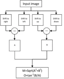
Since SIFTH needs to compute the magnitude and orientation in all pixels in × local window around the keypoints it could decrease the processing time of algorithm. Therefore, we proposed the cascade approach that is shown in Figure 3. In the cascade approach the algorithm select the × local window around each keypoint as input and shift it by one pixel to the left, right, up, and down. In this way algorithm archives all lag factors in Equations (8) and (9). The algorithm could also compute the magnitude and orientation in all pixels by doing just two forwarding steps which are shown in Figure 3. This approach decreases the time of the processing because computing gradient factors in all providing pixels is more beneficial than computing the gradient factors in each pixel separately.
Figure 3. Proposed cascade approach to speed up the computation of orientation.
3.4.2 Orientation Histogram
To form orientation histograms the algorithm classifies the orientations which are obtained in the last phase every 45 degrees, so for covering 360 degrees we achieve 8 classes
which specify the histogram’s bins. For each bin’s magnitude
the algorithm aggregates the magnitudes which are located in the degree class of bin.
Orientation histogram is one of the features of SIFTH descriptor and computed for each × cell in × local window around each keypoint as shown in Figure 4(a).
(a) (b)
Figure 4. (a) The descriptor of SIFTH which has × + = bytes and (b) SIFT descriptor which has ×
= bytes.
3.5 Hue feature extraction
In this phase algorithm computes the average of hue in the × window around each keypoints using following Equation.
� =
∑==− ∑=− − , −(10)
where HueF is the average of hue in the 5×5 window around keypoint, x and y are the location coordinates of the keypoint, and H is the hue of each pixel.
4. DESCRIPTOR FORMATION
To create the descriptor SIFTH divides the × local window around the keypoint into , × windows. Then dominant orientation ∅ which is calculated by Equation (11) is subtracted from each assigned orientation of the pixels of ×
window to resist against rotation of the image. By doing this SIFTH creates the orientation histograms for each × window. Finally the algorithm normalized each histogram to create stable histograms against illumination and contrast changes.
(11)
∅ =
− ∑=− ∑=− � − , − ×� − , −∑=− ∑=− � − , − ×� − , −
where x and y are the location coordinates of the keypoint, H is the hue and I is the illumination of each pixel.
SIFTH descriptor has two features that include orientation histograms and hue feature which are described previously. According to these and Figure 4(a) SIFTH descriptor has , bin orientation histograms and the one byte hue feature. Therefore a single SIFTH descriptor has × + = bytes while SIFT descriptor as shown in Figure 4(b) has , bin orientation histogram which occupied × = bytes.
5. KEYPOINT MATCHING ALGORITHM
In this section at first the algorithm calculates the absolute difference by Equation (12) of hue feature of under processing keypoint and the database of keypoints then if the calculated value were lower than a threshold (we use 0.05) the algorithm keeps keypoint in database if not the keypoint will be eliminated from the probable keypoints.
=
� −
�
(12)
where D is the absolute difference, HueFx is the HueF of under processing keypoint, and HueFt is the HueF of target pixel in database of keypoints.
Then if D were lower than the threshold the matching algorithm calculates the Mean Square Error MSEof orientation histograms using Equation (13).
=
∑ = ∑ = , − ̂ ,
(13)
where m indicates the histogram number, shows the element of histogram, and and ̂ are histograms of two different keypoints.
6. EVALUATIONS
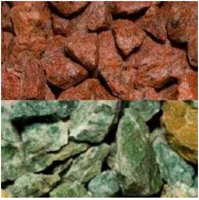
In this section at first we show the data flow of SIFTH by running it on the sample image which is shown in Figure 5.
Figure 5. The sample image for processing.
At the top of the sample image in Figure 5, there is a photo of
“ruby red granite” and at the bottom we see “winter green
granite”.
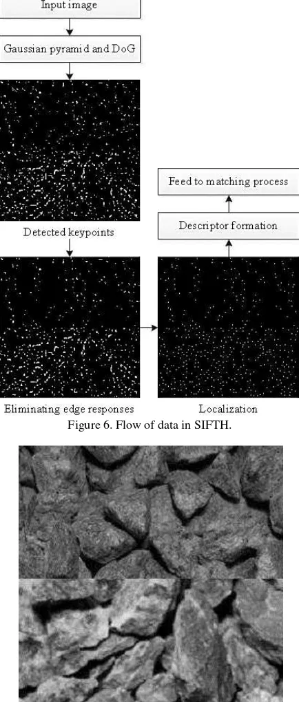
The data flow of SIFTH is shown in Figure 6. As it is shown in Figure 6, number of keypoints after localization phase of SIFTH which is added to SIFT was decreased (for this example it decreased to 468 from 1361), which resulted in decreasing computational load of matching process and lead us to reach real time processing.
The other advantage of SIFTH can be seen in processing of sample image shown in Figure 5. SIFT sees the sample image like what is shown Figure 7. In other words, SIFT does not take
any differences between “ruby red granite” and “winter green
granite” into account. This is originated from the fact that SIFT does not extract any feature related to the color of the under processing image. SIFTH, however, has the hue feature in its descriptor as it is described in section 3.5. Hence, it can detect
the difference between “ruby red granite” and “winter green granite”.
Furthermore, descriptor of SIFTH as discussed in section 4 has bytes consist of × byte of orientation histograms and 1 byte of hue feature. On the other hand, SIFT descriptor has 16×8 byte of orientation histograms which is longer than SIFTH descriptor around two times. This fact also decreases the computational load of matching process.
There is some feature extraction methods which use hue as a feature like [32]. However, SIFTH in comparison to them has focused on decreasing the computational load, space load, and computational complexity of matching process. Furthermore, SIFTH is based on SIFT which its features are invariant to scale; besides adding hue to feature vector of SIFTH makes it hue invariant.
Figure 6. Flow of data in SIFTH.
Figure 7. The way of facing SIFT with sample image which is shown Figure 5.
7. CONCLUSION
In this paper we proposed a new method for image feature extraction called SIFTH which is based on SIFT. The main benefit of SIFTH in comparison to SIFT is that the descriptor
contained hue feature of keypoint which leads the matching process to find the correct match more precisely. In designing SIFTH algorithm we tried to decrease the computational complexity of the feature extraction algorithm and also create descriptor which requires less computational load in matching process.
As it is shown in evaluation section SIFTH decreases the time complexity by decreasing the number of keypoints. Furthermore, it decreases the space complexity by decreasing the size of descriptor. Meanwhile, it has hue in its descriptor which gives the matching process ability of finding different object with same texture such the objects in Figure 5.
8. REFERENCES
1. D. Picard1, M. Cord, and E. Valle, “Study of Sift Descriptors for Image Matching Based Localization in
Urban Street View Context,” in Proceedings of City
Models, Roads and Traffic ISPRS Workshop, ser. CMRT, pp. 193-198, 2009.
2. S. G. Domadia and T. Zaveri, “Comparative Analysis of Unsupervised and Supervised Image Classification
Techniques,” in Proceeding of National Conference on
Recent Trends in Engineering & Technology, , pp 1-5, 2011.
3. C. Harris and M. Stephens, “A Combined Corner and Edge
Detector,” in Alvey Vision Conference, pp. 147-151, 1988. 4. Ashbrook, N. Thacker, P. Rockett, and C. Brown, “Robust Recognition of Scaled Shapes Using Pairwise Geometric Histograms,” in Proceedings of the 6th British Machine Vision Conference, Birmingham, England, pp. 503-512, 1995.
5. S. Belongie, J. Malik, and J. Puzicha, “Shape Matching
and Object Recognition Using Shape Contexts,” IEEE
Transactions on Pattern Analysis and Machine Intelligence, Vol. 2, No. 4, pp. 509-522, 2002.
6. Vardy and F. Oppacher, “A scale invariant local image
descriptor for visual homing,” Lecture notes in Artificial
Intelligence, pp. 362-381, 2005.
7. Anjulan and N. Canagarajah, “Affine invariant feature extraction using symmetry,” Lecture Notes in Computer Science, Vol. 37, No. 8, pp. 332-339, 2005.
8. J. Koenderink and A. van Doorn, “Representation of Local
Geometry in the Visual System,” Biological Cybernetics,
Vol. 55, No. 1, pp. 367-375, 1987.
9. L. Florack, B. ter Haar Romeny, J. Koenderink, and M.
Viergever, “General Intensity Transformations and Second Order Invariants,” in Proceedings of the 7th Scandinavian
Conference on Image Analysis, Aalborg, Denmark, pp. 338-345, 1991.
10. K. Terasawa, T. Nagasaki and T. Kawashima, “Robust matching method for scale and rotation invariant local
descriptors and its application to image indexing,” Lecture
Notes in Computer Science, Vol 36, No. 89, pp. 601-615, 2005.
11. T. Lindeberg, “Feature Detection with Automatic Scale Selection,” International Journal of Computer Vision, Vol. 30, No. 2, pp. 279-116, 1998.
12. T. Linderberg and J. Garding, “Shape-Adapted Smoothing in Estimation of 3-D Shape Cues from Affine Deformations of Local 2-D Brightness Structure,” International Journal of Image and Vision Computing, Vol. 15, No. 6, pp. 415-434, 1997.
13. D. G. Lowe, “Object Recognition from Local Scale
-Invariant Features,” in Proceeding of the 7th International
Conference of Computer Vision, Kerkyra, Greece, pp. 1150-1157, 1999.
14. K. Mikolajczyk, C. Schmid. “Indexing Based on Scale
Invariant Interest Points,” in Proceedings of the 8th
International Conference of Computer Vision, Vancouver, Canada, pp. 525-531, 2001.
15. K. Mikolajczyk and C. Schmid, “An Affine Invariant
Interest Point Detector,” in Proceeding of 7th European Conference of Computer Vision, Copenhagen, Denmark, Vol. 1, No. 1, pp. 128-142, 2002.
16. K. Mikolajczyk and C. Schmid, “Scale and Affine
Invariant Interest Point Detectors,” International Journal of
Computer Vision, Vol. 1, No. 60, pp. 63-86, 2004. 17. Baumberg. “Reliable Feature Matching across Widely
Separated Views,” in Proceeding of Conference on
Computer Vision and Pattern Recognition, Hilton Head Island, South Carolina, USA, pp. 774-781, 2000.
18. F. Schaffalitzky and A. Zisseman. “Multi-View Matching
for Unordered Image Sets,” in Proceedings of the 7th
European Conference on Computer Vision, Copenhagen, Denmark, pp. 414-431, 2002.
19. T. Kadir, M. Brady, and A. Zisserman, “An Affine Invariant Method for Selecting Salient Regions in Images,” in Proceedings of the 8th European Conference on Computer Vision, Prague, Czech Republic, pp. 345-457, 2004.
20. J. Matas, O. Chum, M. Urban, and Y. Pajdle, “Robust Wide Baseline Stereo from Maximally Stable Extremal
Regions,” in Proceedings of the 13th British Machine Vision Conference, Cardiff, UK, pp. 384-393, 2002. 21. Johnson and M. Hebert, “Object Recognition by Matching
Oriented Points,” in Proceedings of Conference on
Computer Vision and Pattern Recognition, Puerto Rico, USA, pp. 684-689, 1997.
22. S. Lazebnik, C. Schmid, and J. Ponce, “Sparse Texture Representation Using Affine-Invariant Neighborhoods,” in Proceedings of Conference on Computer Vision and Pattern Recognition, Madison, Wisconsin, USA, pp. 319-324, 2003.
23. S. Lazebnik, C. Schmid and J. Ponce, “A sparse texture
representation using local affine regions,” IEEE
Transaction on Pattern Analysis and Machine Intelligence, Vol. 27, No. 8, pp. 1265-1278, 2005.
24. R. Zabih and J. Woodfill, “Non-Parametric Local Transforms for Computing Visual Correspondence,” in Proceedings of the 3rd European Conference on Computer Vision, Stockholm, Sweden, pp. 151-158, 1994.
25. D. G. Lowe, “Distinctive Image Features from Scale
-Invariant Interest Point Detectors,” International Journal of
Computer Vision, Vol. 2, No. 60, pp. 91-110, 2004. 26. K. Mikolajczyk and C. Schimd, “A performance evaluation
of local descriptor,” IEEE Transaction on Pattern Analysis
and Machine Learning, Vol. 27, No. 10, pp. 1615-1630, 2005.
27. E. Jauregi, E. Lazkano and B. Sierra, “Object recognition using region detection and feature extraction,” in Proceedings of towards autonomous robotic systems (TAROS), pp. 2041-6407, 2009.
28. Y. Ke and R. Sukthankar, “PCA-SIFT: A More Distinctive
Representation for Local Image Descriptors,” in
Proceeding of Conference on Computer Vision and Pattern Recognition,Washington, USA, pp. 511-517, 2004. 29. N. Chen and D. Blostein, “A survey of document image
classification: problem statement, classifier architecture
and performance evaluation,” International Journal of
Document Analysis & Recognition(IJDAR), Vol. 10, No. 1, pp. 1-16, 2007.
30. G. Fritz, C. Seifert and M. Kumar, “Building detection
from mobile imagery using informative SIFT descriptors,”
Lecture Notes in Computer Science, Vol. 35, No. 40, pp. 629-638, 2005.
31. M. Grabner, H. Grabner and H. Bischof, “Fast
approximated SIFT,” Lecture Notes in Computer Science,
Vol. 38, No. 51, pp. 918-927, 2006.
32. Van de Weijer, Joost, Theo Gevers, and Andrew D.
Bagdanov. “Boosting color saliency in image feature detection.” IEEE transactions on pattern analysis and machine intelligence 28.1. 150-156, 2006.
Referencing books:
33. T. Hastie, R. Tibshirani, and J. Friedman, The Elements of Statistical Learning, Data Mining, Inference, and Prediction, 2nd Ed. Springer Series in Statistics, 2009. The International Archives of the Photogrammetry, Remote Sensing and Spatial Information Sciences, Volume XLII-2/W6, 2017