G.E. Nasr
a,U, E.A. Badr
a, G. Dibeh
ba
Department of Electrical, Computer and Industrial Engineering, Lebanese American Uni¨ersity, 475 Ri¨erside Dr. no. 1846, New York, NY 10115-0065, USA
bDepartment of Economics and Management, Lebanese American Uni¨ersity, 475 Ri¨erside Dr.
no. 1846, New York, NY 10115-0065, USA
Abstract
This paper applies econometric models to investigate determinants of electrical energy
Ž .
consumption in post-war Lebanon. The impact of the Gross Domestic Product GDP ,
Ž . Ž .
proxied by total imports TI , and degree days DD on electricity consumption is investi-gated over different time spans covering the period from 1993 to 1997. The time spans are chosen according to the rationing level of electricity supply. For the 1993]1994 time span,TI
is found to be a significant determinant of energy consumption, whereas, DDhas a negative correlation. This inconsistency might be attributed to an extensive rationing policy followed during this period. For the 1995]1997 time span which includes reduced rationing period
Ž1995 , all electrical energy consumption determinants are found to be significant at the 5%.
significance level. Analysis results for the rationing free 1996]1997 time span also show the
significance of TI and DD at the 5% level. Furthermore, cointegration analysis for the
1995]1997 and 1996]1997 subsets reveals the existence of a long-run relationship between all variables. In addition, error correction models for both subsets are developed to predict short-run dynamics. Finally, statistical performance measures such as mean square error, mean average deviation and mean average percentage error are presented for all models.
Q2000 Elsevier Science B.V. All rights reserved.
JEL classifications:C51; Q41
Keywords:Electricity consumption; Econometric models; Lebanon
U
Corresponding author. Tel.:q1-961-9-547254 ext. 2367; fax:q1-961-9-547256.
Ž .
E-mail address:[email protected] G.E. Nasr .
0140-9883r00r$ - see front matterQ2000 Elsevier Science B.V. All rights reserved.
Ž .
1. Introduction
Econometric models have been developed to forecast energy in many countries. A survey of statistical methods to evaluate urban energy needs is presented by
Ž .
Balocco and Grazzini 1997 . Determinants of energy demand in the literature
Ž . Ž .
include degree days DD temperature by Al-Zayer and Al-Ibrahim 1996 ,
popula-Ž .
tion growth, and oil prices by Majumdar and Parikh 1996 and GDP by Dincer and
Ž . Ž .
Dost 1997 . Moreover, Connor 1996 used neural network models to simulate the impact of various physical and economical variables on electricity and energy
Ž .
production levels. Dahl 1994 , after reviewing 50 studies for energy demand in developing countries, found that the most commonly used modeling techniques for aggregate energy demand are the simple static and the partial adjustment models
ŽPAM . Erdogan and Dahl 1997 investigated the impact of income, price and. Ž .
population on the aggregate, industrial, manufacture and mining sectors of energy
Ž .
in Turkey. Eltony and Hosque 1997 presented a cointegrating relationship for the demand of electricity in Kuwait. Moreover, cointegrating relationships were also
Ž
developed for natural gas and gasoline demand in Kuwait Eltony and Al-Mutairi, .
1995; Eltony, 1996 , cointegration models included price, income and population as explanatory variables. This work is the first to investigate the determinants of
electricity consumption in Lebanon and focuses on the post-war period, 1993]1997.
The Lebanon experienced economic growth rates averaging approximately 5% in the period from 1993 to 1997. Economic growth was concentrated in the construc-tion and public investment sectors. This concentraconstruc-tion is evidenced in the large increases in public investments during this period which averaged approximately
6.7% of GDP in 1994]1996 and in the growth of construction permits that
Ž
increased from 10 614 in 1992 to 17 433 in 1996 Central Bank of Lebanon, .
1993]1997 . This increase in economic activities was also accompanied by
renova-tion of war-damaged buildings and facilities both in the public and private sectors. These developments were accompanied by a major drive to renovate and expand existing national capabilities in electricity production. The Electricite Du Liban
ŽEDL electric utility company has developed a comprehensive plan of investments.
costing approximately $330 million for the renovation and expansion of production capacity up to approximately 1300 MW in order to meet peak demand levels. Moreover, power restructuring and expansion projects have been agreed upon between the government and the World Bank with investment total cost of $486 million. Given these large investment outlays, it is important to study the determi-nants in electricity consumption in the Lebanon in order to provide a better planning and execution of power generation expansion in the future. The electrical
Ž
energy consumption barely balanced the production in pre-war Lebanon prior to .
1975 . During the war, from 1975 to 1992, Lebanon halted all infrastructure expansion and restructuring and was only maintaining pre-war facilities. During and after the war, electricity demand exceeded production capacity, consequently, the EDL implemented a rationing policy. Black outs reached approximately 12 h a
day in 1993]1994 and 6.5 h during 1995. Rationing was almost non-existent starting
Ž Ž ..
Fig. 1. Electrical energy consumption for the period 1993]1997.
Moreover, electricity demand varies during different periods of the year. During
the hot and humid summer, substantial use of ArC equipments is required in the
coastal and heavily populated areas to maintain comfortable indoor spaces. In this
Ž .
paper, the impact and statistical significance of TI GDP proxy and DD on
electrical energy consumption is investigated over different time spans of the
1993]1997 period. Furthermore, the use of the models in forecasting future
electrical energy consumption is investigated.
2. Data and explanatory variables
Monthly data on electricity consumption in Lebanon is obtained from EDL. The Ž .
response, electrical energy consumption C in GW-h, for the whole study period,
1993]1997, is shown in Fig. 1.
Fig. 2. Total imports for the period 1993]1997.
figures in Lebanon are available only on a yearly basis and are highly unreliable. Ž .
Total imports TI are used as a proxy for the GDP for both theoretical and data
availability reasons. Imports are a positive function of the GDP with the rate of change given by the marginal propensity to import out of income making it an ideal
proxy variable for GDP. Moreover, data on TI, shown in Fig. 2, are available at a
higher frequency and are considered to be very reliable.TIdata are obtained from
Ž .
reports of the Central Bank of Lebanon 1993]1997 .
Ž .
The second explanatory variable used in this study is the degree days DD.
Ž .
Heating DD HDD were calculated using:
Ž . Ž .
HDDs
Ý
18.6yTiavg 1i
For any day i of the month with temperature less than 18.68C. Cooling DD
ŽCDD.were calculated using:
Ž . Ž .
CDDs
Ý
Tiavgy23.3 2i
For any day i of the month with temperature higher than 23.38C. A composite
DDfor any month of the year is given by:
Ž .
Fig. 3. Degree days per month for the period 1993]1997.
The daily mean temperatures used to calculate DD are obtained from
climato-Ž .
logical monthly bulletins Ghaddar, 1993]1997 . Fig. 3 shows the variability of DD
throughout each year for the 1993]1997 period.
3. Model specification and methodology
The majority of the studies in the literature have mainly analyzed energy demand in countries experiencing normal economic activities under peaceful and stable conditions. However, the economic dynamics existing in war-ravaged coun-tries, as they enter the post-war era, require special consideration. More specifi-cally, a rationing policy of electrical energy supply might be responsible for varying the impact and statistical significance of customary determinants of energy due to
Ž . Ž
the asynchronous recovery of the private energy consumer and public energy .
supplier sectors. Due to this fact, The 1993]1997 period was divided into three
different time spans each comprising different rationing level:
1. The 1993]1994 period where extensive rationing is implemented.
2. The 1995]1997 period, comprising reduced rationing period, year 1995, and
practically rationing free period, 1996]1997.
3. The 1996]1997 period where rationing is virtually non-existent in major
metropolitan centers.
In this study, a static model is first used to model electrical energy demand. The
Ž .
model relates electrical energy consumption to TI GDP proxy and DD. The
Ž .
Ž .
CtsAtqB TI1 tqB DD2 tqut 4
Where:
Ct s electric consumption;
A s constant;
B1, B2s response coefficients of consumption to explanatory variables;
TI s total imports, 106$;
t
DDt s degree days,8C; and
ut s residual term.
Ž .
The Durbin]Watson DW test is used to check for serial correlation of the
Ž .
residuals. A first order autoregressive term given by Eq. 5 is added as a correction measure in case of rejection of the null hypothesis of no serial correlation.
Ž .
utsruty1qet 5
Ž .
In Eq. 5 ut represents the unconditional residuals, et is the innovation in the
disturbance and r is an estimate of the first-order autocorrelation coefficient. The
resulting non-linear model is solved by applying a Marquardt non-linear least squares method.
Ž .
The second model of this study is the partial adjustment model PAM , which is a dynamic model of the following form:
Ž .
CtsAqB TI1 tqB DD2 tqB C3 ty1qut 6
Where Cty1, is the previous value of electricity consumption and all other
variables are, as defined above. The important feature of this model is its ability to
capture the short-run adjustment in electrical energy to changes in TI and DD.
The use of the lagged-dependent variable as an independent variable necessitates the use of the Durbin-h test, instead of the DW, to check for serial correlation of the residuals. The model is also estimated using OLS.
Given that regression models may produce spurious results when time series are
Ž .
non-stationary Granger and Newbold, 1974 , the variables C,TIand DDare then
Ž .
tested for order of integration using the Dickey]Fuller DF and the augmented
Ž . Ž .
Dickey]Fuller ADF tests Nelson and Plosser, 1982 . The second step is to
determine whether the variables that are difference stationary have a long-run
Ž .
relationship Engle and Granger, 1987 . Two cointegration tests are used in this
Ž . Ž .
study, the Johansen 1988 and Engle and Yoo 1987 test methods. Johansen has
Ž .
proposed a maximum likelihood vector autoregressive VAR procedure as a test Ž .
of cointegration. A likelihood ratio LR , trace statistic, determines whether the hypothesis that a number of cointegrating relations at a certain significance level can be accepted or rejected. Engle and Yoo also developed a two-stage procedure to test and estimate cointegration relationships. In the first stage, a cointegration
Ž .
relationship is estimated using Eq. 4 . Variables are cointegrated if they all have a
Ž . Ž .
unit root, I 1 , and there exist a linear combination of these variables that is I 0 . The first sign indicating cointegration is that the residuals obtained from the
Ž .
k l m
Ž . DCtsDoq
Ý
Dl iDCty1qÝ
D2iDTItyiqÝ
D3iDDDtyiqD u4 tyiqet 7is1 is0 is0
Where D is the first-difference operator. The coefficient of the error, D4,
represents speed of adjustment toward the long-run equilibrium.
4. Results
4.1. The 1993]1994 period
Table 1 shows the estimated results at the 5% significance level for this period. The static model explains 40% of the variation in electricity consumption. The
Ž .
Durbin]Watson DW statistic is in the inconclusive region, at the 1% significance
level, in testing for correlation of the residuals. TI is significant while DD
correlates negatively to consumption with a regression coefficient ofy0.26, which
is obviously the wrong expected sign.
The partial adjustment model does not show any improvement over the static
model explaining 46% in electricity demand. Coefficient onTI is significant at the
5% level, while DD again correlates negatively. The lagged consumption
coeffi-cient is also insignificant. Further analysis of the models on the time span
Table 1
a
Regression analysis results for the 1993]1994 time span
Coefficient Static model Partial adjustment
model
DW orh 1.39 Negative
a
Table 2
a
Regression analysis results for the 1995]1997 time span
Ž .
Coefficient Static model AR 1 model Partial adjustment
model
DW orh 0.43 2.19 Negative
DF y2.82 y6.38 y6.24
Ž .
ADF 1 y2.68 y3.91 y3.82
a
Figures in parentheses are t-statistics.
1993]1994 along cointegration and ECM models is deemed to be unnecessary
because of these results. The results for this period are not surprising considering
the state of power generation capacity in Lebanon during 1993]1994. A widespread
rationing policy was implemented during the war period and overflowed into the
post-war era, specifically, into the 1993]1994 period. This rationing policy was
largely implemented and electricity was supplied for 11.75 h in 1993 and 11.5 h in
Ž .
1994. The electrical energy demand forecasted by Electricite Du Liban 1996 for
1993]1994 is 6306 GW-h for the year 1993 and 6800 GW-h for the year 1994. EDL
was only able to produce 67% of the energy demand for both years. The electrical energy consumption in this period is hence considered supply-driven.
4.2. The 1995]1997 period
Table 2 shows the regression analysis results at the 5% significance level. The static model explains 43% of the variation in electricity demand. The null hypothe-sis of no serial correlation is rejected using the DW statistic. The first-order
Ž . Ž . Ž .
autoregressive model, AR 1 , shown in Eqs. 4 and 5 is used to correct for the Ž .
serial correlation. The DW test for the AR 1 model indicates absence of autocor-Ž .
relation. DF and ADF 1 tests of the residuals from this model indicate stationary Ž .
residuals and integration of zero order, I 0 .
The model explains 89% of the variation in electricity demand. All coefficients
are significant at the 5% level including the first order autoregressive term, r.
Furthermore, DD is found to positively correlate to consumption. The coefficients
Ž .
autocorrelation of the residuals were accounted for, in the AR 1 model, all coefficients become significant at the 5% significance level with the right expected sign. The year 1995 represents a transition period for electricity production.
Rationing hours which attained 12 h a day in 1993]1994 were significantly
decreased during this year to 6.5 h a day. The results agree with many studies Ž
found in the literature indicating the significance and impact of GPD Dincer and
. Ž .
Dost, 1997 and DD Al-Zayer and Al-Ibrahim, 1996 though considered
sepa-rately, on electricity consumption. Specifically, the results indicate that an increase
in GDP and DD implicates an increase in electrical energy consumption.
4.3. The 1996]1997 period
In spite of the rationing hours that existed in 1995, analysis results of the
1995]1997 time period are found to be satisfactory. However, separate analysis for
the 1996]1997 time period is performed since rationing was virtually non-existent
for that period. Table 3 shows regression analysis results at the 5% significance level. The DW statistic for the static model indicates serial correlation of the
residuals. The model R2 is 0.13 and all determinants are insignificant at the 5%
level.TIand DDcoefficients are determined to be 0.22 and 0.39, respectively. The
first order autoregressive model is also utilized to correct for serial correlation of the residuals. The model explains 54% of the variation in electricity demand. Again, all coefficients are significant at the 5% level including the first order
autoregressive term, r. Furthermore, DDexhibits positive correlation to
consump-tion.
The performance of the partial adjustment model for this period appear to be as Ž .
good as the AR 1 model. All coefficients are found to be significant at the 5%
level except for DD. The model explains 46% of the variation in electricity
demand. The null hypothesis of no serial correlation is not rejected using the Ž .
Durbin h test. Again, the DF and ADF 1 tests indicate stationarity and integration Ž .
of zero order, I 0 , of the residuals. TI and DD coefficients are 0.25 and 0.27,
respectively. As rationing hours were virtually non-existent, starting 1996, in most of the country, the electrical energy imbalance of consumption and production was eliminated and electricity consumption started to be demand-driven.
5. Cointegration and error correction models
Table 3
a
Regression analysis results for the 1996]1997 time span
Ž .
Coefficient Static model AR 1 model Partial adjustment
model
Figures in parentheses are t-statistics.
variables for the periods 1995]1997 and 1996]1997 and the subsequent analysis of
cointegration and estimation of Error Correction Models. The results in the levels
and differences for the variables C, TI and DD are reported in Table 4. The
results show that we could not reject the null hypothesis of unit roots for the level series. However, the null hypothesis was rejected for the first differences,
indicat-Ž .
ing that the variables are first-difference stationary, I 1 , for both periods. Given these results, the Johansen, and Engle and Yoo tests are used to check for cointegration. The results of the Johansen cointegration test, which is based on a
Ž .
maximum likelihood vector autoregressive VAR procedure, are shown in Table 5.
Table 4
DF and ADF test for stationarity
Ž .
DF ADF 3
Levels 1st difference Levels 1st difference
0.066434 2.406032 3.76 6.65 At most 2 1996]1997
b d
0.825823 55.64383 29.68 35.65 None
b c
0.511556 17.19485 15.41 20.04 At most 1
b
0.062982 1.431164 3.76 6.65 At most 2
a Ž .
L.R. test indicates 1 cointegrating equation s at 5% significance level.
b Ž .
L.R. test indicated 2 cointegrating equation s at 5% significance level.
c
Denotes rejection of the hypothesis at 5% significance level.
d
Denotes rejection of the hypothesis at 1% significance level.
The trace statistic, L.R. test, indicates the presence of at most one and two
cointegrating equations for 1995]1997 and 1996]1997 subsets, respectively, at the
Ž .
5% significance level. These results are corroborated by the Engle and Yoo 1987 Ž .
procedure for cointegration. The residuals from Eq. 4 for both subsets are tested using DF and ADF tests. Both tests indicate stationary residuals and integration of
Ž .
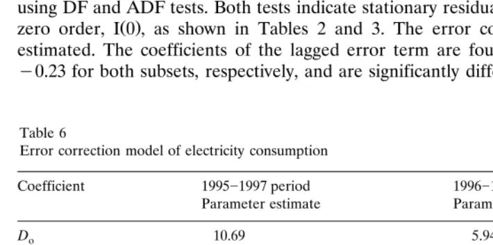
zero order, I 0 , as shown in Tables 2 and 3. The error correction models are
estimated. The coefficients of the lagged error term are found to be y0.18 and
y0.23 for both subsets, respectively, and are significantly different from zero. The
Table 6
Error correction model of electricity consumption
Coefficient 1995]1997 period 1996]1997 period
residuals are stationary and not correlated. The results for the ECM models are shown in Table 6.
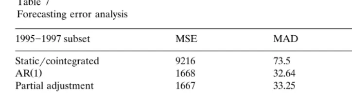
6. Forecasting error analysis
The significant models pertaining to the 1995]1997 and 1996]1997 time spans
are compared. In this work, three statistical measures are used to compare the
Ž .
relative performance of the models. The mean square error MSE is given by:
n
1 2
ˆ
Ž .MSEs
Ý
Ž
CiyCi.
8nis1
The MSE is a useful tool that emphasizes the existence of large residuals even if
Ž .
they are scarce. The mean absolute deviation MAD is given by:
n
The MAD is used to de-emphasize large residuals in case they exist. Finally, the
Ž .
mean absolute percentage error MAPE is given by:
n
ˆ
In the above definitions,Ci, represents the predicted consumption value andCi
represents the actual value. The MAPE implicitly relates the size of the residuals to the actual data points. MAPE is most useful when the units of observations are relatively large. These performance measures serve as guideline to the models’ reliability in generating future forecasts. The MSE, MAD and MAPE for the
different models of the 1995]1997 and 1996]1997 subsets are reported in Table 7.
The models’ forecasting reliability are almost identical.
7. Conclusions
This paper develops three econometric models to investigate the impact of total imports, as a proxy for GDP, and degree days on the demand of electrical energy in
Lebanon for the period 1993]1997. The investigation of the determinants of
electricity consumption in 1993]1994 was unsatisfactory. This shortcoming is due
to long rationing periods that were implemented in addition to the large imbalance
between electrical energy supply and demand. For the 1995]1997 time span, the
static model is corrected for serial correlation of the residuals by including a Ž .
1996]1997 subset
Staticrcointegrated 2955 42.51 6.71
Ž .
AR 1 1522 30.53 4.70
Partial adjustment 1769 31.52 4.90
1995]1997 period exhibits an equally good performance with the exception of the
insignificance of degree days at the 5% level. These plausible results can be attributed to the reduced rationing hours in 1995, making electrical energy
con-sumption demand-driven rather than supply-driven. The analysis of the 1996]1997
time span, prompted by its rationing free status, shows that all determinants are significant at the 5% level except for the lagged term in the partial adjustment model. To account for non-stationarity of the time series as evidenced by the DF and ADF tests, the cointegration hypothesis is tested using the Johansen and Engle and Yoo procedures. Both tests indicate that the variables are cointegrated and
that a long-run relationship exists among them in both 1995]1997 and 1996]1997
subsets. Error correction models for both subsets are developed to predict short-run dynamics. Finally, statistical performance measures for all models in both subsets are calculated.
References
Al-Zayer, J., Al-Ibrahim, A., 1996. Modeling the impact of temperature on electricity consumption in
Ž .
the eastern province of Saudi Arabia. J. Forecast. 15 2 , 97]106.
Balocco, C., Grazzini, G., 1997. A statistical method to evaluate urban energy needs. Int. J. Energy Res.
Ž .
21 14 , 1321]1330.
Central Bank of Lebanon, 1993]1997. Economic Data Reports. Beirut.
Ž .
Connor, J.T., 1996. A robust neural network filter for electricity demand prediction. J. Forecast. 15 6 , 437]458.
Dahl, C., 1994. A survey of energy demand elasticities for the developing world. J. Energy Devel. 1]47.
Ž .
Dincer, I., Dost, S., 1997. Energy and GDP. Int. J. Energy Res. 21 2 , 153]167. Electricite Du Liban, 1996. The Electricity in Lebanon. Eid Press, Beirut.
Eltony, M.N., 1996. Demand for natural gas in Kuwait: an empirical analysis using two econometric models. Int. J. Energy Res. 20, 957]963.
Ž .
Eltony, M.N., Al-Mutairi, N.H., 1995. Demand for gasoline in Kuwait. Energy Econ. 17 3 , 249]253. Eltony, M.N., Hosque, A., 1997. A cointegrating relationship in the demand for energy: the case of
Ž .
electricity in Kuwait. J. Energy Devel. 21 2 , 293]301.
Engle, R.F., Granger, C.W.J., 1987. Co-integration and error correction: representation, estimation and testing. Econometrica 55, 251]276.
Engle, R.F., Yoo, B.S., 1987. Forecasting and testing in cointegrated systems. J. Econometr. 5, 143]159.
Ž .
Ghaddar, N., 1993]1997. American University of Beirut Climatological Data-Monthly Reports. AUB Press, Beirut.
Granger, C.W.J., Newbold, P., 1974. Spurious regressions in econometrics. J. Econometr. 2, 111]120. Johansen, S., 1988. Statistical analysis of cointegration vectors. J. Econ. Dynam. 12, 231]254.
Ž .
Majumdar, S., Parikh, J., 1996. Energy demand forecasts with investment constraints. J. Forecast. 15 6 , 459]476.