Vol. 44 (2001) 221–232
Anticipatory learning in two-person games: some
experimental results
q
Fang-Fang Tang
∗Division of Applied Economics, Nanyang Business School, Nanyang Technical University, Singapore 639798, Singapore
Received 12 October 1998; received in revised form 12 October 1999; accepted 19 October 1999
Abstract
Crawford [Econometrica 42 (1974) 885; J. Econ. Behavior Organ. 6 (1985) 69] has presented a striking example in which plausible adaptive learning rules fail to locate a straightforward mixed-strategy equilibrium. However, Selten [Game Equilibrium Models I. Springer, Berlin 1991, p. 98] argued that such learning rules can be stabilized for some games if there is an anticipation component in the learning process. This paper reports on an experiment designed to test Selten’s predictions. There is evidence in support of Selten’s stability prediction in the sense that the data from a game predicted to be stable comes closer to Nash equilibrium than data from a game predicted to be unstable. © 2001 Elsevier Science B.V. All rights reserved.
JEL classification: C72; C73; C92; D83
Keywords: Mixed Nash equilibrium; Experimental learning; Stability
1. Introduction
Consider a model in which, each period, players from two large populations are randomly matched to play a two-person game in normal form. Between periods, players adjust their behavior in adaptive ways. Assume the game has a unique Nash equilibrium which is completely mixed. For a natural adaptive rule — involving greater player emphasis on better rewarded actions- Crawford (1974, 1985) proved that play will not converge to the equilibrium. This was a striking result. It showed a standard equilibrium to be unstable under a natural adaptive dynamic. Selten (1991), however, rescued stability by hypothesizing that
q
This paper is based on the first chapter of my Ph.D. dissertation, Tang (1996).
∗Fax:+65-791-3697.
E-mail address: [email protected] (F.-F. Tang).
players anticipate and react, still adaptively, to the potential instability. When Selten’s anticipation hypothesis is added to Crawford’s dynamic, the mixed equilibrium becomes stable (for small enough adjustment speeds) if and only if, a certain stability condition on payoffs is met.
In this paper, Selten’s stability condition, and thus, his anticipations hypothesis, is tested experimentally. Two games are specified. One meets Selten’s stability condition and the other does not. The games are roughly similar otherwise. For each game, groups of exper-imental subjects are split into two populations to play the game repeatedly under random matching. Selten’s anticipation hypothesis is supported in the sense that behavior clusters closer to the equilibrium for the game which meets Selten’s stability condition.
Selten’s development is much too long to reproduce. His stability condition can only be sketched. LetAˆbe the normalized payoff matrix faced by a player from the first of the two populations. Here “normalized” means that an appropriate constant is added to each column of the original payoff matrix, say A, to make column sums equal to zero, and an appropriate constant is added to each row of A to make the row sums equal to zero. Similarly, letBˆ be the normalized version of the payoff matrix B, faced by a player from the second of the two populations. Selten’s stability condition is that the non-zero eigenvalues of the matrixAˆBˆT be negative (where T denotes transpose). That is, Selten’s result is this: for small enough adjustment speeds, the mixed equilibrium is stable if and only if the non-zero eigenvalues ofAˆBˆTare negative.
A very rough intuition can be given to the stability condition onAˆBˆT. Selten gives a much longer and more precise intuition. The effect of the first population’s play on the second population’s payoff is determined in substantial part byBˆT, and the effect of the second population’s play on the first population’s payoff is in turn, determined in substantial part by Â. Thus, the effect of the first population’s play on its own payoffs is critically influenced by the product AˆBˆT. Under the adjustment dynamic, negative eigenvalues mean, very roughly speaking, that the first population’s change in mixing probabilities are negatively related to their levels, which creates a stability-promoting effect. From the viewpoint of the second population, a similar interpretation can be given to the transpose ofAˆBˆT. When this stability-promoting effect is present, the instability of the Crawford dynamic is easier to overcome. It turns out that the effect is necessary and sufficient for Selten’s anticipations mechanism to rescue stability. If the game were constant-sum, thenBˆ = − ˆAwould hold, and
ˆ
ABˆT= − ˆAAˆTwould automatically have negative eigenvalues (also see Conlisk 1993a,b). For the two experimental games presented momentarily, the one failing Selten’s stability condition will depart further from constant sums.
Sections 2 and 3 describe the experimental design and procedures. Section 4 describes results. Section 5 concludes the paper.
2. Game design
second game (12.27 and 91.29). That is, Selten’s stability condition is met for the first game and not for the second.
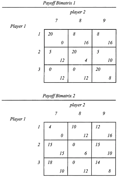
For game 1, by inspection, player 1 likes diagonal cells and player 2 likes off-diagonal cells (somewhat like a poacher-bailiff game, where the three actions are three fish ponds at which player 1, the poacher, does not want to get caught by player 2, the bailiff). For game 2, there is no clear diagonal versus non-diagonal pattern. Also, the payoff sums, cell by cell, are somewhat less variable for game 1 than game 2. Nonetheless, it is not clear from inspection why the first game would have greater stability potential than the second. That is, Selten’s prediction of greater stability for game 1 is not transparent.
Throughout as in the experiment itself, the three actions for player 1 are labelled 1, 2, 3 and for player 2 are labelled 7, 8, 9.
3. Experimental procedure
The experiment was run in the Bonn Experimental Laborotary in 1993. Subjects were recruited by posters from Bonn University; most were law and economics students. No subject participated in more than one session.
Five experimental sessions with 12 subjects in each session were organized for each game. Each session lasted about 2.5 h (one pilot session of 2 h was run 2 weeks before the real sessions). In each session, one game was repeated 150 rounds (except the second and fourth session for game 1, with only 100 rounds, because some subjects spent more time for deliberation during these sessions). Subjects made their decisions at a computer terminal and did not interact in any other way. Before the experiment started, they were instructed with the aid of projector slides about the game and the use of the computer program. Instructions took about 1/2 h and actual play about 2 h. The subjects were also given a one-page reminder of the important information. One protocol, translated into English, is enclosed in Appendix A. The 12 subjects in a session were randomly divided into two groups of six players each so that they formed two “populations”. The first group took the role of player 1, with pure strategy choices 1, 2, 3 while the second group took the role of player 2, with pure strategy choices 7, 8, 9. They were matched randomly by computer at each round to play the game. This set-up was carefully explained to the subjects during the instruction.
The payoffs shown in Fig. 1 are in “points”. On the computer screens, the numbers were in yellow for group 1 and in green for group 2, in blue frames. The exchange rate was 3 Pfennigs per point in the first session for game 1 and 2 Pfennigs per point in the other sessions. (One German Mark equals 100 Pfennigs.) The exchange rate was always clearly announced during the instruction period and was typed in bold letters on the reminder page. The instructor also explicitly reminded the subjects that the amount they earned in the experiment would be paid in cash immediately after the experiment, and that “the more points you get, the more money you get”. The game is easy to understand and the monetary payment is quite attractive compared to the short time span. On average, subjects made about 18 Marks per hour while the student wage rate in Germany was about 11 Marks per hour at that time.
Fig. 1. The games: payoffs are shown at the upper left corner for player 1 and at the lower right corner for player 2. In the experiment, the strategies are labelled 1, 2, 3 for player 1 and 7, 8, 9 for player 2.
choices. When all 12 subjects made up their mind and sent their choices to the network master, the master program calculated each subject’s payoff according to the matching at that round and sent this information back to each subject, respectively. Only the subject knew his or her own payoff for a round. Each subject was also informed about: (i) his or her opponent’s payoff (but not the opponent’s identity), (ii) the average payoffs and choice frequencies in both groups, (iii) the “fictitious-play” expected payoffs of the pure strategies against the other group’s choice distribution and (iv) his or her total points through that round. A “beep” announced the start of the next round.
on-line help function as much as they wanted. About half of the subjects never used this function, and only about a fourth of the subjects used this function repeatedly.
All the irrelevant keys on the computer keyboards were “sealed” by the experimenter. The master program recorded vitually everything the subjects had done on their keyboards and all the information they had seen on their screens. Additionally, each subject was provided with a pencil and one page of blank paper, but only about 20 percent of the subjects ever used the pencil and paper.
All subjects were interviewed, with the help of the laboratory staff, immediately after the experimental sessions, as they were waiting for their payments in cash. The conversations were typewritten later by the experimenter. Subjects talked freely about how they made their choices, what they thought during the game playing, what frequency patterns (if any) they had observed, how they tried to make use of their observations, and so on. All the detailed records are available from the author upon request.
4. Experimental results
4.1. Summary statistics
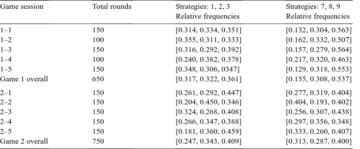
Table 1 gives relative frequencies of pure strategies for the five experimental sessions, for each game. For game 1, subjects in the player 2 population choose among pure strategies 7, 8, and 9 with empirical frequencies close to the theoretical prediction of (1/6, 1/3, 1/2). On the other hand, the player 1 population chooses among the three pure strategies with roughly equal likelihood. Of course, if one population sticks to the equilibrium strategy, the average payoff to the other population is in equilibrium regardless of its strategy. For game 2, neither population is close to the Nash equilibrium frequencies.
Fig. 2 depicts the movement of subjects’ choices over time for the first two sessions for each game. The first two sessions are representative. The data are organized into a sequence of 10-round groups. The points on the graph are aggregate frequencies within a
Table 1
Overview of experimental data
Game session Total rounds Strategies: 1, 2, 3 Strategies: 7, 8, 9 Relative frequencies Relative frequencies
1–1 150 [0.314, 0.334, 0.351] [0.132, 0.304, 0.563]
1–2 100 [0.355, 0.311, 0.333] [0.162, 0.332, 0.507]
1–3 150 [0.316, 0.292, 0.392] [0.157, 0.279, 0.564]
1–4 100 [0.240, 0.382, 0.378] [0.217, 0.320, 0.463]
1–5 150 [0.348, 0.306, 0347] [0.129, 0.318, 0.553]
Game 1 overall 650 [0.317, 0.322, 0.361] [0.155, 0.308, 0.537]
2–1 150 [0.261, 0.292, 0.447] [0.277, 0.319, 0.404]
2–2 150 [0.204, 0.450, 0.346] [0.404, 0.193, 0.402]
2–3 150 [0.324, 0.268, 0.408] [0.256, 0.307, 0.438]
2–4 150 [0.266, 0.347, 0.388] [0.297, 0.356, 0.348]
2–5 150 [0.181, 0.360, 0.459] [0.333, 0.260, 0.407]
10-round group. The notation “10-RA” means “10-round aggregate”. (Similar graphs for the other sessions, and 5-RA and 1-RA graphs for all sessions, are available from the author upon request. Of course, the 5-RA and 1-RA graphs show more variability than the 10-RA graphs.) The left and right graphs are for the player 1 and player 2 populations, respectively. For game 1 (Fig. 2A) the most prominent feature is striking: the frequency curves of strategies 1, 2, and 3 twist around the 1/3 horizontal line, while the frequency curves of strategies 7, 8, and 9 separate clearly, moving around 1/6, 1/3, 1/2, respectively. This pattern is persistent for all five sessions, in the 10 round data aggregation and in the 5 round data aggregation. For game 2 (Fig. 2B) there is no such clear pattern.
Apparently, the Nash equilibrium prediction is not well supported by the data. Then, what do the subjects play? This is a fundamentally difficult question, debated by O’Neill (1987,1991) and Brown and Rosenthal (1990). Every simple theory is wrong, but one might like to know how wrong each theory is. In addition to the Nash model and the random play model, McKelvey and Palfrey (1995) have developed another general framework: the quantal response equilibrium (QRE) for normal form games. QRE is basically a statistical extension of the Nash equilibrium concept gotten by introducing certain error structures. The authors have fit the QRE model to a variety of experimental data sets and found that the QRE model out-performs the Nash or the random play model in most cases. The quantal response model has been fit to the data of this experiment. See Appendix B. In nearly all sessions, the Nash and random predictions can be rejected in favor of the QRE at the 1% level using a likelihood ratio test.
4.2. Test of Selten’s stability prediction
Although subjects do not converge to Nash equilibrium play, we can test Selten’s stability prediction in a weaker sense by asking whether subjects show less variability of behavior in game 1 than in game 2. One approach is to compute variability across sessions. Let (f1,f2,f3) and (f7,f8,f9) be the frequencies across all sessions for the two populations for a given game; and let (x1,x2,x3) and (x7,x8,x9) be the corresponding frequencies for a single session for that game. Then
s=
q
(x1−f1)2+(x2−f2)2+(x3−f3)2+(x7−f7)2+(x8−f8)2+(x9−f9)2
measures the extent to which the particular session varies from the average. There is such a measure for each of the five sessions for game 1 and for each of the five sessions for game 2. The 10 measures are presented on Table 2. It is clear from inspection that there is less variability and greater stability for game 1 than for game 2. As discussed in the footnote to Table 2, the difference is significant by a Wilcoxon test.
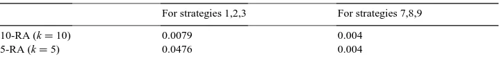
Another approach to testing for stability of behavior is to organize observations within a given session into 10-round groups, as on Fig. 2, and then to look at variability of the 10-round averages relative to the overall average of the session. Let (x,y,z) be the frequencies for a particular session overall, and let (xk,yk,zk) be the frequencies for the kth of the 10-round
groups. Then, letting K be the number of groups,
Table 2
Between-session distance measuresa
Between-session distance measurement of stability
Game 1 Distance Rank Game 2 Distance Rank
Session 1 0.039 2 Session 1 0.081 5
Session 2 0.062 4 Session 2 0.192 10
Session 3 0.059 3 Session 3 0.130 8
Session 4 0.139 9 Session 4 0.092 7
Session 5 0.032 1 Session 5 0.091 6
aWilcoxon test: the sum of rankings for game 1, namelyW=1+2+3+4+9=19 will be this small with
probability P(W≤19)=0.0476. Thus, the null hypothesis of no difference between sessions can be rejected at significance level of 5% in favor of the hypothesis that game 1 is less variable.
Table 3
Within-session distance measuresa
Probability associated with the occurrence of the Wilcoxon statistic under null hypothesis of no difference
For strategies 1,2,3 For strategies 7,8,9
10-RA (k=10) 0.0079 0.004
5-RA (k=5) 0.0476 0.004
aWilcoxon test: in every case, the null hypothesis of no difference can be rejected at significance level of 5%
in favor of the hypothesis that game 1 is less variable.
measures variability within the session in question. As discussed in the footnote to Table 3, the difference is significant by a Wilcoxon test. Similar calculations for five-round groupings lead to the same conclusion.
5. Conclusion
This is the first experimental study to test Selten’s stability prediction for anticipatory learning. Although the experimental behavior does not converge to the Nash equilibrium in either game, Selten’s prediction is qualitatively supported. For the game predicted to be stable, behavior is closer to the equilibrium and is less variable. The result seems striking because the stable game does not appear by inspection to have better stability potential than the unstable game.
Acknowledgements
and an anonymous referee have greatly helped the exposition. Financial support from the Deutsche Forschungsgemeinschaft and the Sonderforschungsbereich 303 is gratefully ac-knowledged. I am greatly indebted to my advisor, Reinhard Selten, whose ideas have shaped this project. Any errors are mine.
Appendix A. Experiment reminder (translated from German, for game 1)
The Game
• Two participants play a game.
• Each must decide to choose one of the three strategies. • One must choose either 1 or 2 or 3.
• The other must choose either 7 or 8 or 9.
• When both participants have made their choices, each will earn the points in the payoff table which has given the decision combinations.
• The first, who chooses either 1 or 2 or 3, earns the point at the upper left corner in the chosen cell. (On the screen, in yellow color.)
• The second, who chooses either 7 or 8 or 9, earns the point at the lower right corner in the chosen cell. (On the screen, in green color.)
• The goal of this game is to make as many points as possible. The example
• If 1 and 7 are chosen, the first earns 20 points and the second earns 0 point. • If 1 and 8 are chosen, the first earns 8 points and the second earns 16 points. • If 1 and 9 are chosen, the first earns 8 points and the second earns 16 points. • If 2 and 7 are chosen, the first earns 5 points and the second earns 12 points. • If 2 and 8 are chosen, the first earns 20 points and the second earns 4 points. • If 2 and 9 are chosen, the first earns 5 points and the second earns 10 points. • If 3 and 7 are chosen, the first earns 0 point and the second earns 12 points • If 3 and 8 are chosen, the first earns 0 point and the second earns 12 points. • If 3 and 9 are chosen, the first earns 20 points and the second earns 8 points.
Experiment structure:
• The twelve participants will be divided into two groups of six each.
• Each participant will stay in the same group throughout the whole experiment. • The participants in group 1 must choose either strategy 1 or 2 or 3.
• Every participant will play 150 rounds.
• In each new round, the participants will be randomly matched, so that there may be always new combinations of the participants from both groups.
Payoff:
• The total winning is the sum of the points in all 150 rounds. • The exchange rate is 2 Pfennig per point.
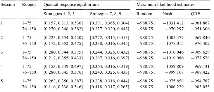
Appendix B
Quantal response equilibrium predictions (by McKelvey and Palfrey) are given in Tables 4 and 5.
Table 4
Game 1: for the first and second half-sessions
Session Rounds Quantal response equilibrium Maximum likelihood estimates
Strategies 1, 2, 3 Strategies 7, 8, 9 Random Nash QRE
1 1–75 [0.307, 0.364, 0.329] [0.152, 0.349, 0.499] −988.751 −972.919 −925.483 76–150 [0.261, 0.356, 0.383] [0.142, 0.344, 0.514] −988.751 −949.189 −925.749 2 1–50 [0.309, 0.364, 0.327] [0.153, 0.349, 0.498] −659.167 −660.167 −635.908 51–100 [0.330, 0.366, 0.303] [0.163, 0.352, 0.485] −659.167 −668.449 −629.574 3 1–75 [0.307, 0.364, 0.329] [0.152, 0.349, 0.499] −988.751 −980.775 −938.491 76–150 [0.240, 0.351, 0.409] [0.141, 0.343, 0.516] −988.751 −941.930 −929.150 4 1–50 [0.187, 0.340, 0.474] [0.154, 0.337, 0.509] −659.167 −621.917 −621.215 51–100 [0.375, 0.358, 0.267] [0.223, 0.357, 0.420] −659.167 −681.495 −654.670 5 1–75 [0.332, 0.366, 0.302] [0.164, 0.352, 0.484] −988.751 −999.688 −929.488 76–150 [0.261, 0.356, 0.383] [0.142, 0.344, 0.514] −988.751 −946.364 −923.711
Table 5
Game 2: for the first and second half-sessions
Session Rounds Quantal response equilibrium Maximum likelihood estimates
Strategies 1, 2, 3 Strategies 7, 8, 9 Random Nash QRE
1 1–75 [0.157, 0.313, 0.530] [0.331, 0.365, 0.304] −988.751 −1031.412 −961.867 76–150 [0.270, 0.348, 0.382] [0.237, 0.320, 0.443] −988.751 −970.297 −951.306
2 1–75 [0.225, 0.354, 0.420] [0.272, 0.315, 0.413] −988.751 −1005.477 −967.840 76–150 [0.172, 0.352, 0.475] [0.338, 0.316, 0.345] −988.751 −1078.015 −976.402
3 1–75 [0.280, 0.344, 0.375] [0.244, 0.325, 0.432] −988.751 −1010.046 −969.629 76–150 [0.212, 0.355, 0.433] [0.287, 0.316, 0.397] −988.751 −1019.986 −977.578
4 1–75 [0.153, 0.349, 0.497] [0.364, 0.316, 0.319] −988.751 −1059.809 −969.131 76–150 [0.280, 0.345, 0.376] [0.243, 0.325, 0.433] −988.751 −999.167 −968.422
References
Brown, J., Rosenthal, R.W., 1990. Testing the minimax hypothesis: a re-examination of O’Neill’s game experiment. Econometrica 58, 1065–1081.
Conlisk, J., 1993a. Adaptation in games: two solutions to the Crawford puzzle. Journal of Economic Behavior and Organization 22, 25–50.
Conlisk, J., 1993b. Adaptive tactics in games: further solutions to the Crawford puzzle. Journal of Economic Behavior and Organization 22, 51–68.
Crawford, V.P., 1974. Learning the optimal strategy in a zero-sum game. Econometrica 42, 885–891.
Crawford, V.P., 1985. Learning behavior and mixed-strategy Nash equilibria. Journal of Economic Behavior and Organization 6, 69–78.
McKelvey, R.D., Palfrey, T.R., 1995. Quantal response equilibria for normal form games. Games and Economic Behavior 10, 6–38.
O’Neill, B., 1987. Nonmetric test of the minimax theory of two-person zerosum games. Proceedings of the National Academy of Science U.S.A. 84, 2106–2109.
O’Neill, B., 1991. Comments on Brown and Rosental’s reexamination. Econometrica 59, 503–507.
Selten, R., 1991. Anticipatory learning in two-person games. In: Selten, R. (Ed.), Game Equilibrium Models I. Springer, Berlin. pp. 98–154.