This art icle was dow nloaded by: [ Universit as Dian Nuswant oro] , [ Ririh Dian Prat iw i SE Msi] On: 01 Oct ober 2013, At : 01: 09
Publisher: Rout ledge
I nform a Lt d Regist ered in England and Wales Regist ered Num ber: 1072954 Regist ered office: Mort im er House, 37- 41 Mort im er St reet , London W1T 3JH, UK
Accounting and Business Research
Publicat ion det ails, including inst ruct ions f or aut hors and subscript ion inf ormat ion: ht t p: / / www. t andf online. com/ loi/ rabr20
Twenty
‐
five years of the Taffler z
‐
score model: Does it
really have predictive ability?
Vineet Agarwal a & Richard J. Taf f ler ba
Cranf ield School of Management and t he Management School, Universit y of Edinburgh, Cranf ield, Bedf ord, MK43 0AL Phone: +44 (0) 1234 751122 Fax: +44 (0) 1234 751122 E-mail:
b
Cranf ield School of Management and t he Management School, Universit y of Edinburgh Published online: 04 Jan 2011.
To cite this article: Vineet Agarwal & Richard J. Taf f ler (2007) Twent y‐f ive years of t he Taf f ler z‐score model: Does it really
have predict ive abilit y?, Account ing and Business Research, 37: 4, 285-300, DOI: 10. 1080/ 00014788. 2007. 9663313
To link to this article: ht t p: / / dx. doi. org/ 10. 1080/ 00014788. 2007. 9663313
PLEASE SCROLL DOWN FOR ARTI CLE
Taylor & Francis m akes every effort t o ensure t he accuracy of all t he inform at ion ( t he “ Cont ent ” ) cont ained in t he publicat ions on our plat form . How ever, Taylor & Francis, our agent s, and our licensors m ake no
represent at ions or warrant ies w hat soever as t o t he accuracy, com plet eness, or suit abilit y for any purpose of t he Cont ent . Any opinions and view s expressed in t his publicat ion are t he opinions and view s of t he aut hors, and are not t he view s of or endorsed by Taylor & Francis. The accuracy of t he Cont ent should not be relied upon and should be independent ly verified w it h prim ary sources of inform at ion. Taylor and Francis shall not be liable for any losses, act ions, claim s, proceedings, dem ands, cost s, expenses, dam ages, and ot her liabilit ies w hat soever or how soever caused arising direct ly or indirect ly in connect ion w it h, in relat ion t o or arising out of t he use of t he Cont ent .
This art icle m ay be used for research, t eaching, and privat e st udy purposes. Any subst ant ial or syst em at ic reproduct ion, redist ribut ion, reselling, loan, sub- licensing, syst em at ic supply, or dist ribut ion in any
1. Introduction
There is renewed interest in credit risk assessment methods following Basel II and recent high profile failures such as Enron and Worldcom. New ap-proaches are continuously being proposed (e.g. Hillegeist et al., 2004; Vassalou and Xing, 2004; Bharath and Shumway, 2004) and academic jour-nals publish special issues on the topic (e.g.
Journal of Banking and Finance, 2001). The tradi-tional z-score technique for measuring corporate financial distress, however, is still a well-accepted tool for practical financial analysis. It is discussed in detail in most of the standard texts and contin-ues to be widely used both in academic literature and by practitioners.
The z-score is used as a proxy for bankruptcy risk in exploring such areas as merger and divest-ment activity (e.g. Shrieves and Stevens, 1979; Lasfer et al., 1996; Sudarsanam and Lai, 2001), asset pricing and market efficiency (e.g. Altman and Brenner, 1981; Katz et al., 1985; Dichev, 1998; Griffin and Lemmon, 2002; Ferguson and
Shockley, 2003), capital structure determination (e.g. Wald, 1999; Graham, 2000; Allayannis et al., 2003; Molina, 2005), the pricing of credit risk (see Kao, 2000 for an overview), distressed securities (e.g. Altman, 2002: ch. 22; Marchesini et al., 2004), and bond ratings and portfolios (e.g. Altman, 1993: ch. 10; Caouette et al., 1998: ch. 19). Z-score mod-els are also extensively used as a tool in assessing firm financial health in going-concern research (e.g. Citron and Taffler, 1992, 2001 and 2004; Carcello et al., 1995; Mutchler et al., 1997; Louwers, 1998; Taffler et al., 2004).
Interestingly, despite the widespread use of the z-score approach, no study to our knowledge has properly sought to test its predictive ability in the almost 40 years since Altman’s (1968) seminal paper was published. The recent paper by Balcaen and Ooghe (2006), which raises a range of impor-tant theoretical issues relating to the model devel-opment process including the definition of failure, problems of ratio instability, sampling bias and choice of statistical method, only serves to demon-strate the need to conduct such empirical tests. The existing literature that seeks to do this, at best, typ-ically uses samples of failed and non-failed firms (e.g. Begley et al., 1996), rather than testing the re-spective models on the underlying population. This, of course, does not provide a true test of ex ante forecasting ability as the key issue of type II error rates (predicting non-failed as failed) is not addressed.1
This paper seeks to fill this important gap in the literature by specifically exploring the question of
Twenty-five years of the Taffler z-score
model: does it really have predictive ability?
Vineet Agarwal and Richard J. Taffler*
Abstract—Although copious statistical failure prediction models are described in the literature, appropriate tests of whether such methodologies really work in practice are lacking. Validation exercises typically use small
sam-ples of non-failed firms and are not true tests of ex ante predictive ability, the key issue of relevance to model users.
This paper provides the operating characteristics of the well-known Taffler (1983) UK-based z-score model for the first time and evaluates its performance over the 25-year period since it was originally developed. The model is shown to have clear predictive ability over this extended time period and dominates more naïve prediction ap-proaches. This study also illustrates the economic value to a bank of using such methodologies for default risk as-sessment purposes. Prima facie, such results also demonstrate the predictive ability of the published accounting numbers and associated financial ratios used in the z-score model calculation.
Keywords: z-scores; bankruptcy prediction; financial ratios; type I and type II errors; economic value
*The authors are, respectively, at Cranfield School of Management and the Management School, University of Edinburgh. They are particularly indebted to the editor, Pauline Weetman, and the anonymous referee for helping them strengthen the paper significantly, as well as their many colleagues and seminar and conference participants, including those at the Financial Reporting and Business Communications Conference, University of Cardiff, July 2004, the European Financial Management Association Conference, Madrid, July 2006, and the American Accounting Association Annual Meeting, Washington, August 2006, who have provided valuable comments on earlier drafts. Correspondence should be addressed to Vineet Agarwal at Cranfield School of Management, Cranfield, Bedford MK43 0AL. Tel: +44 (0) 1234 751122, Fax: +44 (0) 1243 752554, Email: vineet.agarwal@cranfield.ac.uk
This paper was accepted for publication in June 2007.
1The only possible exception is the recent paper of Beaver
et al. (2005) for US data. However, their out-of-sample testing is for a much shorter period than this study, and their focus is not on the predictive ability of published operational models.
whether a well-established and widely-used UK-based z-score model driven by historic accounting data has true ex ante predictive ability over the 25 years since it was originally developed.
The remainder of the paper is structured as fol-lows. Section 2 provides a brief overview of con-ventional z-score methodology and describes the UK-based model originally published in this jour-nal (see Taffler, 1983), including the provision of the actual model coefficients for the first time, which is the subject of our analysis. Section 3 pro-vides our empirical results and tests whether this z-score model really does capture risk of corporate failure. Section 4 reviews issues relating to the temporal stability of z-score models and Section 5 discusses common misperceptions relating to what such models are and are not. The final section, Section 6, provides some concluding reflections.
2. The z-score model
The generic z-score is the distillation into a single measure of a number of appropriately chosen fi-nancial ratios, weighted and added. If the derived z-score is above a cut-off, the firm is classified as financially healthy, if below the cut-off, it is viewed as a potential failure.
This multivariate approach to failure prediction was first published almost 40 years ago with the eponymous Altman (1968) z-score model in the US, and there is an enormous volume of studies applying related approaches to the analysis of cor-porate failure internationally.2This paper reviews the track record of a well-known UK-based z-score model for analysing the financial health of firms listed on the London Stock Exchange which was originally developed in 1977; a full descrip-tion is provided in Accounting and Business Research volume 15, no. 52 (Taffler, 1983). The model itself was originally developed to analyse industrial (manufacturing and construction) firms only with separate models developed for retail and service enterprises.3 However, we apply it across all non-financial listed firms in the performance tests below.4
As explained in Taffler (1983), the first stage in building this model was to compute over 80 care-fully selected ratios from the accounts of all listed industrial firms failing between 1968 and 1976 and 46 randomly selected solvent industrial firms.5 Then using, inter alia, stepwise linear discriminant analysis, the z-score model was derived by deter-mining the best set of ratios which, when taken to-gether and appropriately weighted, distinguished optimally between the two samples.6
If a z-score model is correctly developed its component ratios typically reflect certain key di-mensions of corporate solvency and performance.7 The power of such a model results from the appro-priate integration of these distinct dimensions
weighted to form a single performance measure, using the principle of the whole being worth more than the sum of the parts.
Table 1 provides the Taffler (1983) model’s ratio definitions and coefficients. It also indicates the four key dimensions of the firm’s financial profile that are being measured by the selected ratios. These dimensions, identified by factor analysis, are: profitability, working capital position, finan-cial risk and liquidity. The relative contribution of each to the overall discriminant power of the model is measured using the Mosteller-Wallace criterion. Profitability accounts for around 50% of the discriminant power of the model and the three balance sheet measures together account for a sim-ilar proportion.
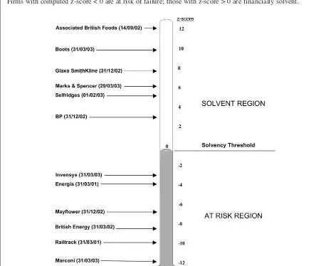
In the case of this model, if the computed z-score is positive, i.e. above the ‘solvency threshold’ on the ‘solvency thermometer’ of figure 1, the firm is solvent and is very unlikely indeed to fail within the next year. However, if its z-score is negative, it lies in the ‘at risk’ region and the firm has a finan-cial profile similar to previously failed businesses and, depending on how negative, a high probabili-ty of financial distress. This may take the form of administration (Railtrack and Mayflower), re-ceivership (Energis), capital reconstruction (Marconi), rescue rights issue, major disposals or spin-offs to repay creditors (Invensys), govern-ment rescue (British Energy), or acquisition as an alternative to bankruptcy.
Various statistical conditions need to be met for valid application of the methodology.8In addition, alternative statistical approaches such as quadratic discriminant analysis (e.g. Altman et al., 1977), logit and probit models (e.g. Ohlson, 1980;
2For example, Altman and Narayanan (1997) review 44
separate published studies relating to 22 countries outside the US.
3Taffler (1984) also describes a model for analysing retail
firms. His unpublished service company model is similar in form.
4 Altman’s (1968) model was also originally developed
from samples of industrial companies alone but has conven-tionally been applied across the whole spectrum of non-finan-cial firms.
5Although smaller than samples currently used in building
failure prediction models, the model was constructed using all firms failing subsequent to the Companies Act, 1967, which significantly increased data availability.
6 Data was transformed and Winsorised and differential
prior probabilities and misclassification costs were taken into account in deriving an appropriate cut-off between the two groups. The Lachenbruch (1967) hold-out test provided two apparent classification errors.
7Factor analysis of the underlying ratio data should be
un-dertaken to ensure collinear ratios are not included in the model leading to lack of stability and sample bias, and to help interpret the resulting model component ratios.
8These are discussed in Taffler (1983) with regard to the
model described here and more generally in Taffler (1982), Jones (1987) and Keasey and Watson (1991) and need not de-tain us here.
Table 1
Model for analysing fully listed industrial firms
The model is given by:
z = 3.20 + 12.18*x1+ 2.50*x2– 10.68*x3+ 0.029*x4 where
x1 = profit before tax/current liabilities (53%) x2 = current assets/total liabilities (13%) x3 = current liabilities/total assets (18%) x4 = no-credit interval1(16%)
The percentages in brackets after the variable descriptors represent the Mosteller-Wallace contributions of the ratios to the power of the model. Via factor analysis, x1measures profitability, x2working capital position,
x3financial risk and x4liquidity.
1no-credit interval = (quick assets – current liabilities)/daily operating expenses with the denominator proxied by (sales –
PBT – depreciation)/365
Figure 1
The Solvency Thermometer
Firms with computed z-score < 0 are at risk of failure; those with z-score > 0 are financially solvent.
Zmijewski, 1984; Zavgren, 1985), mixed logit (Jones and Hensher, 2004), recursive partitioning (e.g. Frydman et al., 1985), hazard models (Shumway, 2001; Beaver et al., 2005) and neural networks (e.g. Altman et al., 1994) are used. However, since the results generally do not differ from the conventional linear discriminant model approach in terms of accuracy, or may even be in-ferior (Hamer, 1983; Lo, 1986; Trigueiros and Taffler, 1996), and the classical linear discriminant approach is quite robust in practice (e.g. Bayne et al., 1983) associated methodological considera-tions are of little importance to users.
3. Forecasting ability
Since the prime purpose of z-score models, implic-itly or explicimplic-itly, is to forecast future events, the only valid test of their performance is to measure their true ex ante prediction ability.9This is rarely done and when it is, such models may be found lacking. This could be because significant num-bers of firms fail without being so predicted (type I errors). However, more usually, the percentage of firms classified as potential failures that do not fail (type II errors) in the population calls the opera-tional utility of the model into question.10In addi-tion, statistical evidence is necessary that such models work better than alternative simple strate-gies (e.g. prior year losses). Testing models only on the basis of how well they classify failed firms is not the same as true ex ante prediction tests.11
3.1. What is failure?
A key issue, however, is what is meant by corpo-rate failure. Demonstrably, administration, re-ceivership or creditors’ voluntary liquidation constitute insolvency.12 However, there are alter-native events which may approximate to, or are clear proxies for, such manifestations of outright failure and result in loss to creditors and/or share-holders. Capital reconstructions, involving loan write-downs and debt-equity swaps or equivalent, can equally be classed as symptoms of failure, as can be acquisition of a business as an alternative to bankruptcy or major closures or forced disposals of large parts of a firm to repay its bankers. Other symptoms of financial distress, more difficult to identify, may encompass informal government support or guarantees, bank intensive care moni-toring or loan covenant renegotiation for solvency reasons, etc. Nonetheless, in the analysis in this paper, we work exclusively with firm insolvencies on the basis these are clean measures, despite probably weakening the apparent predictive abili-ty of the z-score model, in particular in terms of in-creasing the type II error rate.
3.2. The population risk profile
To assess the z-score model’s performance in
practical application, z-scores for the full popula-tion of non-financial firms available electronically and fully listed on the London Stock Exchange for at least two years at any time between 1979 (sub-sequent to when the model was developed) and 2003, a period of 25 years, are computed.13,14 During this period there were 232 failures in our sample; 223 firms (96.1%) had z-scores < 0 based on their last published annual accounts prior to failure indicating they had potential failure pro-files.15The average time to failure from the date of the last annual accounts is 13.2 months, similar to that reported by Ohlson (1980) for the US.16The equivalent median figure is 13.0 months.
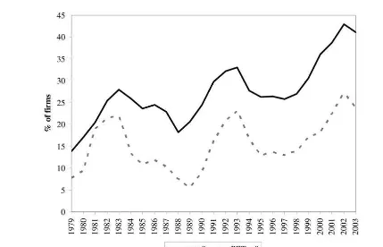
Figure 2 shows the percentage of firms in our sample with negative z-scores and percentage of firms with negative PBT both of which vary over time. In the case of z-scores, the low of 14% is
reg-9Whereas techniques such as the Lachenbruch (1967)
jack-knife method, which can be applied to the original data to test for search and sample bias, are often used, inference to per-formance on other data for a future time period cannot be made because of potential lack of population stationarity.
10 For example, the Bank of England model (1982) was
classifying over 53% of its 809 company sample as potential failures in 1982, soon after it was developed.
11Good examples are Begley et al. (1996) who conduct
out-of-sample tests of type I and type II error rates for 1980s fail-ures for both the Altman (1968) and Ohlson (1980) models and Altman (2002: 17–18) who provides similar sample statis-tics for his 1968 model through to 1999. However, neither
study allows the calculation of true ex ante predictive ability,
the acid test of such model purpose, because the full popula-tion of non-failed firms is not considered.
12The term bankruptcy, used in the US, applies only to
per-sons in the UK.
13 The required accounting data was primarily collected
from the Thomson Financial Company Analysis and EXSTAT
financial databases which between them have almost complete coverage of UK publicly fully listed companies. For the small
number of cases not covered, MicroEXSTATand Datastream
were also used in that order. We have assumed a lag of five months between the balance sheet date and public availability of the annual accounts.
14Altman (1993) claims that a respecification of his 1968
z-score model recalculated using his original sample of publicly traded firms but substituting the book value of equity for mar-ket value in his ratio 4 can be applied to non-listed firms. However, this is incorrect. The financial profiles of privately owned firms differ significantly to those of listed firms. As such, models need to be developed directly from samples of failed and non-failed non-listed firms. It would be invalid to apply the z-score model described here to such entities.
15Of the nine firms misclassified, six had negative z-scores
on the basis of their latest available interim/preliminary ac-counts prior to failure. On this basis, only three companies could not have been picked up in advance, including Polly Peck, where there were serious problems with the published accounts. Among other issues, there is a question mark over a missing £160m of cash and even the interim results, published only 17 days before Polly Peck’s shares were suspended, show profits before tax of £110m on turnover of £880m. Whereas, as argued below, such multivariate models are quite robust to window dressing, this obviously cannot apply to major fraud.
16The z-score becomes negative on average 2.4 years
(me-dian = 2.0) before failure. The equivalent PBT figures are 1.4 (1.0) years respectively.
istered in 1979 and the graph peaks at 43% in 2002, higher than the peaks of 33% in 1993 and 28% in 1983 at the depths of the two recessions. The overall average is 27%. The percentage of firms with negative profit before tax (PBT) shows a similar time-varying pattern but is lower with an overall average of 15%.
3.3. True ex ante predictive ability
We use two different methods to assess the power of such models to capture the risk of financial dis-tress – tests of information content and tests of pre-dictive ability. Three alternative classification rules are employed for statistical comparison – a propor-tional chance model which randomly classifies all firms as failures or non-failures based on ex post
population failure rates, a naïve model that classi-fies all firms as non-failures and a simple account-ing-based model that classifies firms with negative PBT as potential failures and those with PBT>0 as non-failures.17Also, misclassification costs need to be properly taken into account. In addition, we need to consider if the magnitude of the negative
z-score has further predictive content.
3.3.1. Relative information content tests
As illustrated above, z-scores are widely used as a proxy for risk of failure. It is therefore important to test if they carry any information about the probability of failure and, hence, whether it is jus-tified to use them as a proxy for bankruptcy risk. We also test whether the same information can be captured by our simple prior-year loss-based clas-sification rule.
To test for information content, a discrete hazard model of the form similar to that of Hillegeist et al. (2004) is used:
(1)
where:
pi,t = probability of failure of firm i in year t, X = column vector of independent variables,
and
β = column vector of estimated coefficients. This expression is of the same form as logistic regression; Shumway (2001) shows that it can be estimated as a logit model. However, the standard
Figure 2
Percentage of firms at risk
Z-scores and PBT figures for all the firms in our sample are computed based on their full-year accounts with financial year-ends between May 1978 and April 2004. The figures for year t are based on full-year accounts of all the firms in the sample with balance sheet dates between May of year t–1 and April of year t.
17The authors are indebted to Steven Young for this
sugges-tion.
errors will be biased downwards since the logit es-timation treats each firm year observation as inde-pendent, while the data has multiple observations for the same firm. Following Shumway (2001) we divide the test statistic by the average number of observations per firm to obtain an unbiased statis-tic.
We estimate two models; model (i) with z-score dummy (0 if negative, 1 otherwise) and model (ii) with PBT dummy (0 if negative, 1 otherwise) as independent variables. The dependent variable is the actual outcome (1 if failed, 0 otherwise). The parametric test of Vuong (1989) is used to test whether the log-likelihood ratios of our two logit models differ significantly. Table 2 provides the results.
Coefficients on both z-score in model (i) and PBT in model (ii) are significant at better than the 1% level showing both variables carry significant information about corporate failure. However, the coefficient on z-score (–4.2) is much larger than that on PBT (–2.5) even though they are both measured on the same scale of 0 to 1 and the log-likelihood statistic for model (i) is smaller than that for model (ii) demonstrating that, on this basis, the z-score carries more information about
failure than does PBT. The difference between the two log-likelihood statistics is statistically signifi-cant (Vuong test statistic = 4.62; p<0.01).
These results show that our z-scores do carry in-formation about corporate failure and are thus a valid proxy for risk of financial distress. They also show that z-score dominates PBT.
3.3.2. Test of predictive ability
Only a proportion of firms at risk, however, will suffer financial distress. Knowledge of the popula-tion base rate allows explicit tests of the true ex ante predictive ability of the failure prediction model where the event of interest is failure in the next year. We use the usual 2x2 contingency table approach to assess whether our two accounting-based models, z-score and prior-year loss, do bet-ter than the proportional chance model.
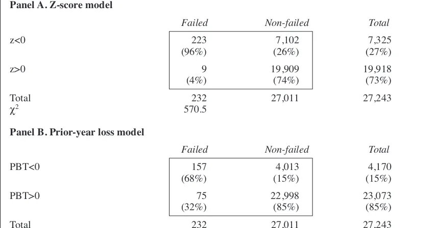
The contingency table for z-score is provided in panel A of Table 3. It shows that of the 232 failures in our sample; 223 firms (96.1%) had z-scores < 0 based on their last accounts prior to failure indicat-ing they had potential failure profiles. In total, over the 25-year period, there were 7,325 (27%) firm years with z<0 and 19,918 (73%) with z>0. The overall conditional probability of failure given a negative z-score is 3.04% (223/7,325). This differs significantly to the base failure rate of 0.85% (232/27,243) at better than α= 0.001 (z = 20.4).18 Similarly, the conditional probability of non-failure given a positive z-score is 99.95% (19,909/19,918),
Table 2
Relative information content
Z-score and PBT figures for all the firms in our sample are computed based on their last available full-year ac-counts with financial year-ends from May 1978 until April 2004. Firms are then tracked till delisting or publi-cation of their next full-year accounting statements to identify those that failed. The z-score model classifies all firms with z<0 as potential failures and the PBT model classifies all firms with PBT<0 as potential failures. Figures in brackets are the Wald statistic from the logistic regression with dependent variable taking a value of 1 if the firm fails subsequent to its last available annual accounts, 0 otherwise. The Wald and model χ2
statis-tics are adjusted for the fact that there are several observations from the same firm by dividing by 10.74, the average number of observations per firm.
Variable Model (i) Model (ii)
Constant –3.46 –3.24
(241.12) (147.75)
PBT –2.49
(28.75)
Z-score –4.24
(14.46)
Model χ2 48.40 30.41
Log-likelihood –1077 –1173
Pseudo-R2 0.20 0.13
With 1 degree of freedom, critical Wald and χ2values at 1%, 5% and 10% level are 6.63, 3.84 and 2.71
respectively.
18 z=(p–π)/冪——π(1–π)/———nwhere p = sample proportion, π =
probability of chance classification and n = sample size. For the conditional probability of failure given z<0, p = 0.0304, π = 0.0085 and n = firms with z<0 = 7,325.
which differs significantly from the base rate of 99.15% at better than α = 0.001 (z = 12.4).19 In addition, the computed χ2 statistic is 570.5 and strongly rejects the null hypothesis of no associa-tion between failure and z-score. Thus, the z-score model possesses true forecasting ability on this basis.
Panel B of Table 3 provides the results of using prior year loss as the classification criteria. It shows that 68% of the 232 failures over the 25-year period registered negative PBT on the basis of their last accounts before failure. In total there were 4,170 (15%) firm years with PBT<0 and 23,073 (85%) with PBT>0. On this basis, the over-all conditional probability of failure given a nega-tive PBT is 3.76% (157/4,170), which differs significantly to the base failure rate of 0.85% at better than α= 0.001 (z = 20.5).20 Similarly, the
conditional probability of non-failure given a pos-itive PBT is 99.67% (22,998/23,073), which dif-fers significantly from the base rate of 99.15% at better than α= 0.001 (z = 8.7).21The χ2statistic is 495.0 and strongly rejects the null hypothesis of no association between failure and loss in the last year. On this basis, a simple PBT-based model also appears to have true forecasting ability.
These results confirm the evidence of Table 2, both z-scores and PBT have true failure forecast-ing ability, however, they do not directly indicate which of the two models is superior.
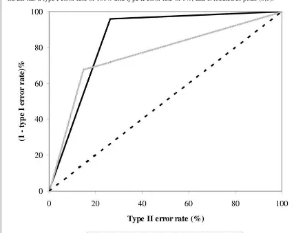
3.3.3. Comparing the predictive ability of z-scores and PBT using the ROC curve
The Receiver Operating Characteristics (ROC) curve is widely used for assessing various rating methodologies (see Sobehart et al., 2000 for de-tails). It is constructed by plotting 1 – type I error rate against the type II error rate and the model with larger area under the curve (AUC) is consid-ered to be a better model. The Gini coefficient or accuracy ratio is just a linear transformation of the area under the ROC curve, i.e.:
Gini coefficient = 2*(AUC – 0.50) (2)
The area under the ROC curve is estimated using the Wilcoxon statistic following Hanley and
Table 3
Classification matrix for z-scores and prior-year losses
Z-score and PBT figures for all the firms in our sample are computed based on their last available full-year ac-counts with financial year-ends from May 1978 until April 2004. Firms are then tracked till delisting or publi-cation of their next full-year accounting statements to identify those that failed. The z-score model classifies all firms with z<0 as potential failures and the PBT model classifies all firms with PBT<0 as potential failures. The null hypothesis of no association between z (PBT) and failure is tested using the χ2statistic.
Panel A. Z-score model
Failed Non-failed Total
z<0 223 7,102 7,325
(96%) (26%) (27%)
z>0 9 19,909 19,918
(4%) (74%) (73%)
Total 232 27,011 27,243
χ2 570.5
Panel B. Prior-year loss model
Failed Non-failed Total
PBT<0 157 4,013 4,170
(68%) (15%) (15%)
PBT>0 75 22,998 23,073
(32%) (85%) (85%)
Total 232 27,011 27,243
χ2 495.0
19For the conditional probability of non-failure given z>0 at
the beginning of the year, p = 0.9995, π= 0.9915 and n =
19,918.
20 z=(p–π)/冪——π(1–π)/———nwhere p = sample proportion, π =
probability of chance classification and n = sample size. For the conditional probability of failure given PBT<0, p = 0.0376,
π= 0.0085 and n = firms with PBT<0 = 4,170.
21 For the conditional probability of non-failure given
PBT>0 at the beginning of the year, p = 0.9967, π= 0.9915
and n = 23,073.
McNeil (1982) who demonstrate that it is an unbi-ased estimator (also see Faraggi and Reiser, 2002). The standard error of area under the ROC curve is given by (Hanley and McNeil, 1982):
(3)
where:
A = area under the ROC curve,
nF = number of failed firms in the sample, nNF = number of non-failed firms in the sample, Q1 = A/(2–A), and
Q2 = 2A2/ (1+A)
and the test statistic is:
(4)
where z is a standard normal variate.
To compare the AUC for two different models, the test statistic is:22
(5)
where again z is the standard normal variate. Figure 3 plots the AUC for the z-score and PBT models with the diagonal line representing the pro-portional chance model, while the AUC for the naïve model will be zero (i.e. (0,0)).23 Figure 3 shows that the z-score model has a larger AUC (0.85) than the PBT model which in turn has a larg-er AUC (0.76) than the proportional chance model. Table 4 presents summary statistics and shows that both z-score and PBT models outperform the proportional chance model (z = 21.9 and 14.4 re-spectively). It also shows that the z-score model outperforms the PBT model (z = 3.5). On this basis, while both z-score and PBT perform better than random classification, again the z-score model clearly outperforms the PBT model.
3.3.4. Differential error costs
All the tests presented so far assume the cost of misclassifying a firm that fails (type I error) is the same as the cost of misclassifying a firm that does not fail (type II error). However, in the credit mar-ket, the cost of a type I error is not the same as the
cost of a type II error. In the first case, the lender can lose up to 100% of the loan amount while, in the latter case, the loss is just the opportunity cost of not lending to that firm. In assessing the practi-cal utility of failure prediction models’ ability, then, differential misclassification costs need to be explicitly taken into account.
Blöchlinger and Leippold (2006) provide a framework to assess the economic utility of differ-ent credit risk prediction models in a competitive loan market. The following assumptions apply for an illustrative accept/reject cut-off regime:24
1. Banks use a model to either accept or reject customers.
2. The risk premium is exogenous (75 basis points), i.e. all customers that are accepted will be offered the same rate.
3. The loss from lending to a customer that de-faults is 40% of the loan amount.
4. A customer will randomly select a bank for his/her loan application. If this application is rejected, he/she will then randomly select an-other bank, and so on until the loan is granted.
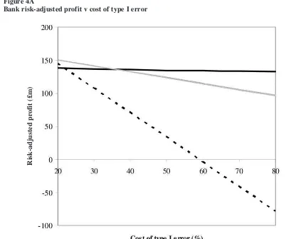
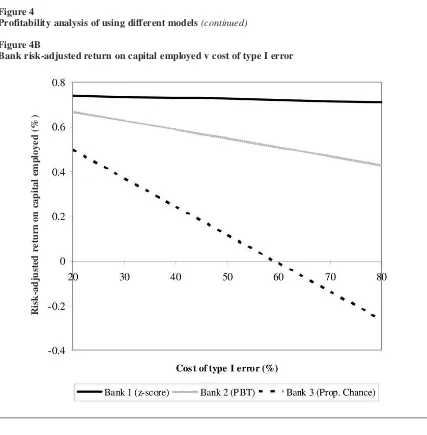
For our analysis, we assume there are four banks in the market with total loan demand of £100bn. Without loss of generality we further assume all loans are of the same amount and for a one-year period. Bank 1 uses the z-score model for making loan decisions (accept all customers with z-score > 0, reject all others), Bank 2 employs the prior-year loss model (accept all customers with PBT > 0, re-ject all others), Bank 3 uses the proportional chance model (i.e. randomly accept or reject customers based on overall failure rate) and Bank 4 adopts a naïve approach (i.e. accept all customers). Table 5 provides the summary statistics for the four banks. Table 5 shows that while Bank 1 which employs the z-score model has the smallest market share (19%), it has loans of the best credit quality with a default rate of just 1%. This rate compares to that of 11% for Bank 2. Bank 1 also earns higher prof-its that any other bank despite having the smallest loan portfolio and outperforms the next best, Bank 2, by 24% (14 basis points in absolute terms) in terms of risk-adjusted return on capital employed. Figure 4 provides a sensitivity analysis for the different models as the cost of a type I error changes. Figure 4A plots profitability and shows that the proportional chance model generates lower profits than the PBT model for the cost of a type I error in the range of 20% to 80% and gener-ates lower profits than the z-score model for a type I error cost in excess of 22%. It also shows that the z-score model leads to higher profits than the PBT model for cost of a type I error in excess of 36%. Figure 4B plots the risk-adjusted return on capital employed (ROCE) and shows that the z-score
22Hanley and McNeil (1983) propose an adjustment for the
fact that the two AUCs are derived from the same data and will therefore be correlated. The effect of this induced correlation will be to reduce the standard error. Our test statistics which ignore this are therefore conservative.
23The proportional chance model randomly classifies firms
as failed/non-failed based on the population failure rate while the naïve model classifies all firms as non-failed.
24Although this regime may appear an oversimplification,
this is exactly how the credit insurance market works in prac-tice.
model dominates the other two models across the entire range of type I error costs with the differ-ence in the risk adjusted ROCE between z-score and PBT models ranging from 7 to 28 basis points. In relative terms, this gives z-score risk adjusted profitability outperformance of between 10% and 65%.25The economic benefit of using the z-score model in this illustrative setting is thus clear.
3.3.5. Probability of failure and severity of negative z-score
Most academic research in this field has focused exclusively on whether the derived z-score is above or below a particular cut-off. However, does the magnitude of the (negative) z-score provide further information on the actual degree of risk of failure within the next year for z<0 firms?
To explore whether the z-score construct is an ordinal or only a binary measure of bankruptcy risk, we explore failure outcome rates by negative z-score quintiles over our 25-year period. Table 6 provides the results.
Figure 3 ROC curves
Z-score and PBT figures for all the firms in our sample are computed based on their last available full-year accounts with financial year-ends from May 1978 until April 2004. Firms are then tracked till delisting or pub-lication of their next full-year accounting statements to identify those that failed. The z-score model classifies all firms with z<0 as potential failures, the PBT model classifies all firms with PBT<0 as potential failures, the proportional chance model randomly classifies firms as failed/non-failed based on overall failure rate for our sample period (0.85%) and the naïve model classifies all firms as non-failed. The type I error rate for the z-score (prior-year loss) model is computed as the number of failed firms with positive z-score (PBT) divided by the total number of failures. The type II error rate for the z-score (prior-year loss) model is computed as the number of non-failed firms with negative z-score (PBT) divided by the total number of non-failures. The re-spective type I and type II error rates for the proportional chance model are 99.15% and 0.85%. The naïve model has a type I error rate of 100% and type II error rate of 0%, and is located at point (0,0).
25Blöchlinger and Leippold (2006) show in their simulation
models that these results are lower bound estimates; in more complex settings, the profitability differences are likely to be larger.
Table 4
ROC curves: summary statistics
Z-score and PBT figures for all the firms in our sample are computed based on their last available full-year ac-counts with financial year-ends from May 1978 until April 2004. Firms are then tracked till delisting or publi-cation of their next full-year accounting statements to identify those that failed. The z-score model classifies all firms with z<0 as potential failures and the PBT model classifies all firms with PBT<0 as potential failures. The AUC is estimated as a Wilcoxon statistic, and the Gini coefficient (Gini) is derived from the AUC using equation (2) in the text. The standard error (se) of the AUC is estimated using equation (3), and the z-statistic (z) for the test of significance of the AUC is estimated using equations (4) and (5) in the text.
AUC se z Gini
Z-score 0.85 0.0159 21.9 0.70
PBT 0.76 0.0184 14.4 0.53
Difference 0.09 0.0243 3.5
Table 5
Bank profitability using different models
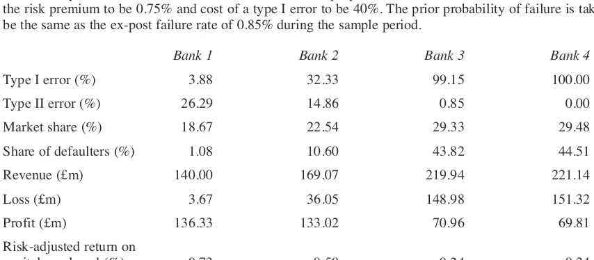
Z-score and PBT figures for all the firms in our sample are computed based on their last available full-year ac-counts with financial year-ends from May 1978 until April 2004. Firms are then tracked till delisting or publi-cation of their next full-year accounting statements to identify those that failed. Bank 1 uses the z-score model that classifies all firms with z<0 as potential failures, Bank 2 employs the PBT model which classifies all firms with PBT<0 as potential failures, Bank 3 adopts the proportional chance model that randomly classifies firms as potentially failed/non-failed based on the average failure rate over the 25-year period (0.85%) and Bank 4 classifies all firms as non-failures using the naïve model. Firms are assumed to randomly choose one of the four banks and if rejected by the first bank, then randomly select one of the other three banks and so on until the loan is granted. The type I error rate represents the percentage of failed firms classified as non-failed by the respective model, and the type II error rate represents the percentage of non-failed firms classified as failed by the respective model. Market share is the expected number of (equal size) loans granted as a percentage of total number of firm years, share of defaulters is the expected number of defaulters to whom a loan is granted as a percentage of total number of defaulters. Revenue is calculated as market size * market share * risk premium and loss is calculated as market size * prior probability of failure * share of defaulters * cost of a type I error in percent. Profit is calculated as revenue – loss. Risk adjusted return on capital employed is calculated as prof-it divided by market size * market share. For illustrative purposes, we assume the market size to be £100bn, the risk premium to be 0.75% and cost of a type I error to be 40%. The prior probability of failure is taken to be the same as the ex-post failure rate of 0.85% during the sample period.
Bank 1 Bank 2 Bank 3 Bank 4
Type I error (%) 3.88 32.33 99.15 100.00
Type II error (%) 26.29 14.86 0.85 0.00
Market share (%) 18.67 22.54 29.33 29.48
Share of defaulters (%) 1.08 10.60 43.82 44.51
Revenue (£m) 140.00 169.07 219.94 221.14
Loss (£m) 3.67 36.05 148.98 151.32
Profit (£m) 136.33 133.02 70.96 69.81
Risk-adjusted return on
capital employed (%) 0.73 0.59 0.24 0.24
Figure 4
Profitability analysis of using different models
Z-score and PBT figures for all the firms in our sample are computed based on their last available full-year ac-counts with financial year-ends from May 1978 until April 2004. Firms are then tracked till delisting or publi-cation of their next full-year accounting statements to identify those that failed. Bank 1 uses the z-score model that classifies all firms with z<0 as potential failures, Bank 2 employs the PBT model which classifies all firms with PBT<0 as potential failures, Bank 3 adopts the proportional chance model that randomly classifies firms as potentially failed/non-failed based on the average failure rate over the 25-year period (0.85%) and Bank 4 classifies all firms as non-failures using the naïve model. Firms are assumed to randomly choose one of the four banks and if rejected by the first bank, then randomly select one of the other three banks and so on until the loan is granted. Market share is the expected number of (equal size) loans granted as a percentage of total number of firm years, share of defaulters is the expected number of defaulters to whom a loan is granted as a percentage of total number of defaulters. Revenue is calculated as market size * market share * risk premium and loss is calculated as market size * prior probability of failure * share of defaulters * cost of a type I error in percent. Profit is calculated as revenue – loss. Risk-adjusted return on capital employed is calculated as prof-it divided by market size * market share. A type I error is classifying a failed firm as non-failed, and a type II error is classifying a non-failed firm as failed by the respective model. For illustrative purposes, we assume the market size to be £100bn and the risk premium to be 0.75%. Figure 4A plots bank risk-adjusted profits and Figure 4B bank risk-adjusted return on capital employed both against cost of a type I error in percent. The cor-responding figures for Bank 4 (naïve model) are always less than those for Bank 3 (proportional chance model) and omitted from the graphs for ease of exposition.
Figure 4A
Bank risk-adjusted profit v cost of type I error
R
is
k
-ad
ju
ste
d
p
rofi
t (£m)
Figure 4
Profitability analysis of using different models(continued)
Figure 4B
Bank risk-adjusted return on capital employed v cost of type I error
R
is
k
-ad
ju
ste
d
r
etu
rn
on
c
ap
ital
e
mp
loye
d
(%)
Table 6
Firm failure probabilities by negative z-score quintile
Z-score and PBT figures for all the firms in our sample are computed based on their last available full-year ac-counts with financial year-ends from May 1978 until April 2004. Each year, the firms are ranked on their z-scores based on the full-year accounts with financial year ending between May of year t–1 and April of year t. For the negative z-score stocks, five portfolios of equal number of stocks are formed each year. Firms are then tracked till delisting or publication of their next full-year accounting statements to identify those that failed. The z-score model classifies all firms with z<0 as failures. Entries in the table refer exclusively to the –ve z-score firms in our sample.
Negative z-score quintile (t–1)
Outcome (t) 5 (worst) 4 3 2 1 (best) Total firms
Failed (%) 7.1 4.1 2.0 1.3 0.7 223
Non-failed (%) 92.9 95.9 98.0 98.7 99.3 7,102
Number of firms 1,475 1,467 1,466 1,460 1,457 7,325
% of total failures (n = 232) 44.8 25.9 12.9 8.2 4.3 96.1
As can be seen, there is a monotononic relation-ship between severity of z-score and probability of failure in the next year which falls from 7.1% in the worst quintile of z-scores to 0.7% for the least negative quintile. Overall, the weakest 20% of negative z-scores accounts for 45% of all failures and the lowest two quintiles together capture over two thirds (71%) of all cases. A contingency table test of association between z-score quintile and failure rate is highly significant (χ2= 133.0).26As such, we have clear evidence the worse the nega-tive z-score, the higher the probability of failure; the practical utility of the z-score is clearly signif-icantly enhanced by taking into account its magni-tude.
4. Temporal stability
Mensah (1984) points out that users of accounting-based models need to recognise that such models may require redevelopment from time to time to take into account changes in the economic envi-ronment to which they are being applied. As such, their performance needs to be carefully monitored to ensure their continuing operational utility. In fact, when we apply the Altman (1968) model originally developed using firm data from 1945 to 1963 to non-financial US firms listed on NYSE, AMEX and NASDAQ between 1988 and 2003, we find almost half of these firms (47%) have a z-score less than Altman’s optimal cut-off of 2.675. In addition, 19% of the firms entering Chapter 11 during this period had z-scores greater than 2.675.27
Nonetheless, it is interesting to note that, in prac-tice, such models can be remarkably robust and continue to work effectively over many years, as convincingly demonstrated above. Altman (1993: 219–220) reports a 94% correct classification rate for his ZETA™ model for over 150 US industrial bankruptcies over the 17-year period to 1991, with 20% of his firm population estimated as then
hav-ing ZETA™ scores below his cut-off of zero. In the case of the UK-based z-score model re-viewed in this paper, Figure 2 shows how the per-centage of firms with at-risk z-scores varies broadly in line with the state of the economy. However, it increases dramatically from around 26% in 1997 to 41% by 2003.28
Factors that might be driving this increase in negative z-score firms in the recent period include (i) the growth in the services sector associated with contraction in the number of industrial firms listed, (ii) the doubling in the rate of loss-making firms between 1997 and 2002, as demonstrated in Figure 2, with one in four firms in 2002 making historic cost losses, even before amortisation of goodwill, (iii) increasing kurtosis in the model ratio distribu-tions indicating reduced homogeneity in firm fi-nancial structures, and (iv) increasing use of new financial instruments (Beaver et al., 2005). There are also questions about the impact of significant changes in accounting standards and reporting practices over the life of the z-score model, al-though as the model is applied using accounting data on a standardised basis, any potential impact of such changes is reduced.
Begley et al. (1996) and Hillegeist et al. (2004) recalculate Altman’s original 1968 model updating his ratio coefficients on new data; however, both papers find that their revised models perform less well than the original model. The key requirement is to redevelop such models using ratios that meas-ure more appropriately the key dimensions of firms’ current financial profiles reflecting the changed nature of their financial structures, per-formance measures and accounting regimes.
Although our results appear to be in contrast to Beaver et al. (2005), who claim their derived three variable financial ratio predictive model is robust over a 40-year period, their only true ex ante tests are based on a hazard model fitted to data from 1962 to 1993 which is tested on data over the fol-lowing eight years. As such, the authors are only in a position to argue for short-term predictive abili-ty. Interestingly, their hazard model also performs significantly less well than the z-score model reported in this paper over a full 25-year out-of-sample time horizon.29
5. Z-score models: discussion
Z-scores, for some reason, appear to generate a lot of emotion and attempts to demonstrate they do not work (e.g. Morris, 1997). However, much of the concern felt about their use is based on a mis-understanding of what they are and what they are designed to do.
5.1. What a z-score model is
Strictly speaking, what a z-score model asks is ‘does this firm have a financial profile more
simi-26The area under the ROC curve when using z-score
quin-tiles is 0.90 and the corresponding accuracy ratio (Gini coeffi-cient) is 0.80. The finer gradation enhances the power of the model since the area under the curve is significantly larger than when using the binary measure (z = 2.6). The details are omitted to save space but are available from the first author on request.
27Begley et al. (1996) report out-of-sample type I and type
II error rates of 18.5% and 25.1% for the Altman (1968) model and 10.8% and 26.6% for the Ohlson (1980) model using small samples of bankrupt and non-bankrupt firms.
28Model users may wish to make a small ad hoc adjustment
of –1.0 to the cut-off from 1997 to account for this in practical application. The type I error rate from 1997 to 2003 does not change but the average type II error rate falls from 35% to 29%. Reducing the cut-off further to –2.0 raises the type I error rate to 15.5% from 11.3% while reducing type II errors to 24%.
29Beaver et al. (2005) also do not take into account
differ-ential error misclassification costs.
lar to the failed group of firms from which the model was developed or the solvent set?’ As such, it is descriptive in nature. The z-score model is made up of a number of fairly conventional finan-cial ratios measuring important and distinct facets of a firm’s financial profile, synthesised into a sin-gle index. The model is multivariate, as are a firm’s set of accounts, and is doing little more than reflecting and condensing the information they provide in a succinct and clear manner.
The z-score is primarily a readily interpretable communication device, using the principle that the whole is worth more than the sum of the parts. Its power comes from considering the different as-pects of economic information in a firm’s set of ac-counts simultaneously, rather than one at a time, as with conventional ratio analysis. The technique quantifies the degree of corporate risk in an inde-pendent, unbiased and objective manner. This is something that is difficult to do using judgement alone. Clearly, to be of value, a z-score model must demonstrate true ex antepredictive ability.
5.2. Lack of theory
Z-score models are also commonly censured for their perceived lack of theory. For example, Gambling (1985: 420) entertainingly complains that:
‘… this rather interesting work (z-scores) … provides no theory to explain insolvency. This means it provides no pathology of organization-al disease … Indeed, it is as if medicorganization-al research came up with a conclusion that the cause of dying is death … This profile of ratios is the cor-porate equivalent of … ‘‘We’d better send for his people, sister’’, whether the symptoms arise from cancer of the liver or from gunshot wounds.’
However, once again, critics are claiming more for the technique than it is designed to provide. Z-scores are not explanatory theories of failure (or success) but pattern recognition devices. The tool is akin to the medical thermometer in indicating the probable presence of disease and assisting in tracking the progress of and recovery from such organisational illness. Just as no one would claim this simple medical instrument constitutes a scien-tific theory of disease, so it is only misunderstand-ing of purpose that elevates the z-score from its simple role as a measurement device of financial risk, to the lofty heights of a full-blown theory of corporate financial distress.
Nonetheless, there are theoretical underpinnings to the z-score approach, although it is true more re-search is required in this area. For example, Scott (1981) develops a coherent theory of bankruptcy and, in particular, shows how the empirically de-termined formulation of the Altman et al. (1977)
ZETA™ model and its constituent variable set fits the postulated theory quite well. He concludes (p.341) ‘Bankruptcy prediction is both empirically feasible and theoretically explainable’. Taffler (1983) also provides a theoretical explanation of the model described in this paper and its con-stituent variables drawing on the well-established liquid asset (working capital) reservoir model of the firm which is supplied by inflows and drained by outflows. Failure is viewed in terms of exhaus-tion of the liquid asset reservoir which serves as a cushion against variations in the different flows. The component ratios of the model measure differ-ent facets of this ‘hydraulic’ system.
There are also sound practical reasons why this multivariate technique works in practice. These re-late to (i) the choice of financial ratios by the methodology which are less amenable to window dressing by virtue of their construction, (ii) the multivariate nature of the model capitalising on the swings and roundabouts of double entry, so manip-ulation in one area of the accounts has a counter-balancing impact elsewhere in the model, and (iii) generally the empirical nature of its development. Essentially, potential insolvency is difficult to hide when such ‘holistic’ statistical methods are ap-plied.
6. Concluding reflections
This study describes a widely-used UK-based z-score model including publication of its ratio coef-ficients for the first time and explores its track record over the 25-year period since it was devel-oped. We believe this is the first study to conduct valid tests of the true predictive ability of such models explicitly. The paper demonstrates that the z-score model described, which was developed in 1977, has true failure prediction ability and typi-fies a far more profitable modelling framework for banks than alternative, simpler approaches. Such z-score models, if carefully developed and tested, continue to have significant value for financial statement users concerned about corporate credit risk and firm financial health. They also demon-strate the predictive ability of the underlying finan-cial ratios when correctly read in a holistic way. The value of adopting a formal multivariate ap-proach, in contrast to ad hoc conventional one-at-a-time financial ratio calculation in financial analysis, is evident.
Z-score models, despite their long history and continuing extensive use by practitioners and re-searchers, still generate much heat among academ-ics, who sometimes appear to be less concerned about practical relevance than elegant economic theory. The widespread theoretical arguments in favour of market based option pricing models (e.g. Kealhofer, 2003; Vassalou and Xing, 2004), such as those provided commercially by Moody’s KMV
(see Saunders and Allen, 2002: 46–64 for more de-tails) are illustrative of this, despite there being no evidence of their superior performance in the bankruptcy prediction task compared with the sim-ple z-score approach (see e.g. Hillegeist et al., 2004; Reisz and Perlich, 2004; Agarwal and Taffler, 2007). Researchers and practitioners are advised to subject all such modelling approaches first to thorough empirical testing as in this paper. A final point relates to the continued misunder-standing of the specific nature of z-score models which can only be appropriately applied to the population of firms from which they were devel-oped. As such, it is totally wrong and potentially dangerous to seek to apply the very accessible Altman (1968) US model in market environments such as the UK. It would be similarly inappropri-ate to draw any inferences from seeking to apply the listed firm z-score model described in this paper to UK privately-owned firms which have very different financial characteristics. Separate models need to be developed for analysing the fi-nancial health of unlisted firms. Falkenstein et al. (2000) show that the distributional properties of listed and private firm ratios are significantly dif-ferent and conclude (p.46):
‘A model fit using public data will deviate sys-tematically and adversely from a model fit using private data, as applied to private firms.’
In addition, seeking to update the coefficients of such models using recent data is unlikely to im-prove their classificatory ability as any redevel-oped z-score model component ratios need to reflect the current key dimensions of firm financial profiles, and ratio set and coefficient estimates need to be jointly determined. If such models start to show signs of age, albeit their longevity as demonstrated empirically in this paper can be im-pressive, then completely new z-score models should be developed unconstrained by prior model ratios.
References
Agarwal, V. and Taffler, R.J. (2007). ‘Comparing the per-formance of market-based and accounting-based bank-ruptcy prediction models’. Journal of Banking and Finance, forthcoming.
Allayannis, G., Brown, G.W. and Klapper, L.F. (2003). ‘Capital structure and financial risk: evidence from for-eign debt use in East Asia’. Journal of Finance, 58(6): 2667–2709.
Altman, E.I. (1968). ‘Financial ratios, discriminant analy-sis and the prediction of corporate bankruptcy’. Journal of Finance, 23(4): 589–609.
___________. (1993). Corporate financial distress and bankruptcy. New York: John Wiley, 2nd edition. ___________. (2002). Bankruptcy, credit risk, and high
yield junk bonds: a compendium of writings. Oxford: Blackwell Publishing.
___________, Haldeman, R.G. and Narayanan, P. (1977).
‘ZETA analysis: A new model to identify bankruptcy risk of corporations’. Journal of Banking and Finance, 1(1): 29–51.
____________ and Brenner, M. (1981). ‘Information ef-fects and stock market response to signs of firm deterio-ration’. Journal of Financial and Quantitative Analysis, 16(1): 35–52.
___________, Marco, G. and Varetto, F. (1994). ‘Corporate distress diagnosis: comparisons using linear discriminant analysis and neural networks (the Italian ex-perience)’. Journal of Banking and Finance, 18(3): 505–529.
___________ and Narayanan, P. (1997). ‘An international survey of business failure classification models’.
Financial Markets and Institutions, 6(2): 1–57.
Balcaen, S. and Ooghe, H. (2006). ‘35 years of studies on business failure: an overview of the classic statistical methodologies and their related problems’. British Accounting Review, 38: 63–93.
Bank of England. (1982). ‘Techniques for assessing corpo-rate financial strength’. Bank of England Quarterly Bulletin, June: 221–223.
Bayne, C.K., Beauchamp, J.J., Kane, V.E. and McCabe, G.P. (1983). ‘Assessment of Fisher and logistic linear and quadratic discriminant models’. Computational Statistics and Data Analysis, 1: 257–273.
Beaver, W.H., McNichols, M.F. and Rhie, J. (2005). ‘Have financial statements become less informative? Evidence from the ability of financial ratios to predict bankruptcy’.
Review of Accounting Studies, 10(1): 93–122.
Begley, J., Ming, J. and Watts, S. (1996). ‘Bankruptcy clas-sification errors in the 1980s: an empirical analysis of Altman’s and Ohlson’s models’. Review of Accounting Studies, 1(4): 267–284.
Bharath, S.T. and Shumway, T. (2004). ‘Forecasting Default with the KMV-Merton Model’. Working paper, University of Michigan.
Blöchlinger, A. and Leippold, M. (2006). ‘Economic bene-fit of powerful credit scoring’. Journal of Banking and Finance, 30: 851–873.
Caouette, J.B., Altman, E.I. and Narayanan, P. (1998).
Managing credit risk: the next great financial challenge. New York: John Wiley and Sons.
Carcello, J.V., Hermanson, D.R. and Huss, H.F. (1995). ‘Temporal changes in bankruptcy-related reporting’. Auditing: A Journal of Practice and Theory, 14(2): 133–143.
Citron, D.B. and Taffler, R.J. (1992). ‘The audit report under going concern uncertainties: an empirical analysis’.
Accounting and Business Research, 22(88): 337–345. ________________________. (2001). ‘Ethical behaviour
in the U.K. audit profession: the case of the self-fulfilling prophecy under going-concern uncertainties’. Journal of Business Ethics, 29(4): 353–363.
________________________. (2004). ‘The comparative impact of an audit report standard and an audit going-con-cern standard on going-congoing-con-cern disclosure rates’.
Auditing: A Journal of Practice and Theory, 23(2): 119–130.
Dichev, I.D. (1998). ‘Is the risk of bankruptcy a systemat-ic risk?’Journal of Finance, 53(3): 1131–1147.
Falkenstein, E., Boral, A. and Carty, L.V. (2000). ‘RiskCalc for private companies: Moody’s default model’. Moody’s Risk Management Services – special comment.
Faraggi, D. and Reiser, R. (2002). ‘Estimation of the area under the ROC curve’. Statistics in Medicine, 21: 3093–3106.
Ferguson, M.F. and Shockley R.L. (2003). ‘Equilibrium “anomalies”’. Journal of Finance, 58(6): 2549–2580.
Frydman, H., Altman, E.I. and Kao, D.G. (1985). ‘Introducing recursive partitioning for financial classifi-cation: the case of financial distress’. Journal of Finance, 40(1): 269–291.
Gambling, T. (1985). ‘The accountant’s guide to the galaxy including the profession at the end of the universe’.
Accounting Organisations and Society, 10(4): 415–426. Graham, J.R. (2000). ‘How big are the tax benefits of
debt?’Journal of Finance, 55(5): 1901–1941.
Griffin, J. and Lemmon, L. (2002). ‘Book-to-market equi-ty, distress risk, and stock returns’. Journal of Finance, 57(5): 2317–2336.
Hamer, M. (1983). ‘Failure prediction: sensitivity of classi-fication accuracy to alternative statistical methods and variable sets’. Journal of Accounting and Public Policy, 2(4): 289–307.
Hanley, J. and McNeil, B. (1982). ‘The meaning and use of the area under a receiver operating characteristic (ROC) curve’. Radiology, 143 (1): 29–36.
Hanley, J. and McNeil, B. (1983). ‘A method of comparing the areas under receiver operating characteristic curves derived from the same cases’. Radiology, 148 (3): 839–843.
Hillegeist, S.A., Keating, E.K., Cram, D.P. and Lundstedt, K.G. (2004). ‘Assessing the probability of bankruptcy’.
Review of Accounting Studies, 9(1): 5–34.
Jones, F.L. (1987). ‘Current techniques in bankruptcy pre-diction’. Journal of Accounting Literature, 6: 131–164. Jones, S. and Hensher, D.A. (2004). ‘Predicting firm
finan-cial distress: a mixed logit model’. The Accounting Review, 79(4): 1011–1038.
Journal of Banking and Finance (2001). Special issue on credit ratings and the proposed new BIS guidelines on capital adequacy for bank credit assets. 25(1).
Kao, D.L. (2000). ‘Estimating and pricing credit risk: an overview’. Financial Analysts Journal, 56(4): 50–66. Katz, S., Lilien, S. and Nelson, B. (1985). ‘Stock market
behaviour around bankruptcy model distress and recovery predictions’. Financial Analysts Journal, 41(1): 70–74. Kealhofer, S. (2003). ‘Quantifying credit risk I: default
pre-diction’. Financial Analysts Journal, 59(1): 30–44. Keasey, K. and Watson, R. (1991). ‘Financial distress
pre-diction models: a review of their usefulness’. British Journal of Management, 2(2): 89–102.
Lachenbruch, P.A. (1967). ‘An almost unbiased method of obtaining confidence intervals for the probability of mis-classification in discriminant analysis’. Biometrics, 23(4): 639–645.
Lasfer, M., Sudarsanam, P.S. and Taffler, R.J. (1996). ‘Financial distress, asset sales, and lender monitoring’.
Financial Management, 25(3): 57–66.
Lo, A.W. (1986). ‘Logit versus discriminant analysis’.
Journal of Econometrics, 31(2): 151–178.
Louwers, T.J. (1998). ‘The relation between going-concern opinions and the auditor’s loss function’. Journal of Accounting Research, 36(1): 143–156.
Marchesini, R., Perdue, G. and Bryan, V. (2004). ‘Applying bankruptcy prediction models to distressed high yield bond issues’. Journal of Fixed Income, 13(4): 50–56.
Mensah, Y. (1984). ‘An examination of the stationarity of multivariate bankruptcy prediction models: a method-ological study’. Journal of Accounting Research, 22(1): 380–395.
Molina, C.A. (2005). ‘Are firms underleveraged? An
ex-amination of the effect of leverage on default probabili-ties’. Journal of Finance, 60(3): 1427–1459.
Morris, R. (1997). Early warning indicators of corporate failure. Ashgate Publishing.
Mutchler, J.P., Hopwood, W. and McKeown, J.C. (1997). ‘The influence of contrary information and mitigating factors on audit opinion decisions on bankrupt compa-nies’. Journal of Accounting Research, 35(2): 295–301. Ohlson, J.A. (1980). ‘Financial ratios and the probabilistic
prediction of bankruptcy’. Journal of Accounting Research, 18(1): 109–131.
Reisz, A. and Perlich, C. (2004). ‘A market based frame-work for bankruptcy prediction’. Working paper, Baruch College, City University of New York.
Saunders, A. and Allen, L. (2002). Credit risk measure-ment: new approaches to value at risk and other para-digms, 2nd edition, Wiley Finance.
Scott, J. (1981). ‘The probability of bankruptcy: a compar-ison of empirical predictions and theoretical models’.
Journal of Banking and Finance, 5: 317–334.
Shrieves, R.E. and Stevens, D.L. (1979). ‘Bankruptcy avoidance as a motive for merger’. Journal of Financial and Quantitative Analysis, 14(3): 501–515.
Shumway, T. (2001). ‘Forecasting bankruptcy more accu-rately: a simple hazard model’. Journal of Business, 74(1): 101–124.
Sobehart J., Keenan, S., Stein, R. (2000). ‘Benchmarking quantitative default risk models: a validation methodolo-gy’. Moody’s Rating Methodology.
Sudarsanam, S. and Lai, J. (2001). ‘Corporate financial dis-tress and turnaround strategies: an empirical analysis’.
British Journal of Management, 12(3): 183–199. Taffler, R.J. (1982). ‘Forecasting company failure in the
UK using discriminant analysis and financial ratio data’.
Journal of Royal Statistical Society, Series A, 145(3): 342–358.
_________. (1983). ‘The assessment of company solvency and performance using a statistical model’. Accounting and Business Research, 15(52): 295–308.
_________. (1984). ‘Empirical models for the monitoring of UK corporations’. Journal of Banking and Finance, 8(2): 199–227.
_________, Lu, J. and Kausar, A. (2004). ‘In denial? Stock market underreaction to going-concern audit report dis-closures’. Journal of Accounting & Economics, 38(1–3): 263–296.
Trigueiros, D. and Taffler, R.J. (1996). ‘Neural networks and empirical research in accounting’. Accounting and Business Research, 26(4): 347–355.
Vassalou, M. and Xing, Y. (2004). ‘Default risk in equity returns’. Journal of Finance, 59 (2): 831–868.
Vuong, Q. (1989). ‘Likelihood ratio tests for model selec-tion and non-nested hypotheses’. Econometrica, 57: 307–333.
Wald, J.K. (1999). ‘How firm characteristics affect capital structure: an international comparison’. Journal of Financial Research, 22(2): 161–187.
Zavgren, C.V. (1985). ‘Assessing the vulnerability to fail-ure of American industrial firms: a logistic analysis’.
Journal of Business Finance and Accounting, 12(1): 19–45.
Zmijewski, M.E. (1984). ‘Methodological issues related to the estimation of financial distress prediction models’.
Journal of Accounting Research, 22 (Supplement): 59–82.