MARKOV CHAIN SMALL-WORLD MODEL WITH
ASYMMETRIC TRANSITION PROBABILITIES∗
JIANHONG XU†
Abstract. In this paper, a Markov chain small-world model of D.J. Higham is broadened by incorporating asymmetric transition probabilities.Asymptotic results regarding the transient behavior of the extended model, as measured by its maximum mean first passage time, are established under the assumption that the size of the Markov chain is large.These results are consistent with the outcomes as obtained numerically from the model.
The focus of this study is the effect of a varying degree of asymmetry on the transient behavior which the extended model exhibits.Being a quite interesting consequence, it turns out that such behavior is largely influenced by the strength of asymmetry.This discovery may find applications in real-world networks where unbalanced interaction is present.
Key words. Asymmetry, Small-world, Ring network, Markov chain, Mean first passage time.
AMS subject classifications.05C50, 15A51, 60J20, 60J27, 65C40.
1. Introduction. First we briefly describe the Markov chain small-world model of a ring network originally proposed by Higham [9]. For background material on the small-world phenomenon,we refer the reader to [13,14,15].
Consider a ring network consisting ofN+ 1 vertices,which are labeled clockwise
as 0, . . . , N. Initially,each vertex is connected to its neighboring vertices1by directed
edges. A one-dimensional symmetric periodic random walk is then introduced on such a ring network. Specifically,starting from any vertex,the process moves to any of the neighboring vertices with equal probability 1/2 over one time unit,thus leading to a homogeneous ergodic Markov chain with state space S ={0, . . . , N} and transition
∗Received by the editors October 6, 2008.Accepted for publication November 11, 2008.Handling Editor: Michael Neumann.
†Department of Mathematics, Southern Illinois University Carbondale, Carbondale, Illinois 62901, USA ([email protected]).
1For any specified vertex, this term refers to the two nearest neighboring vertices on the ring network.
matrix
P0=
0 p p
p . .. ...
. .. ... ... . .. ... p
p p 0
∈R(N+1)×(N+1),
wherep= 1/2.
To model the small-world phenomenon on the ring network,the above Markov chain is modified by also allowing the process to jump to non-neighboring vertices with some small probability ǫ. For such a modified Markov chain,the transition matrix becomes
Pǫ=
ǫ p ǫ · · · p
p . .. ... ...
ǫ . .. ... ...
..
. . .. ... ... p
p p ǫ
∈R(N+1)×(N+1),
where 0< ǫ≤ N1−1 and p= 1
2[1−(N−1)ǫ]. We comment that the idea of adding long-range random jumps to non-neighboring vertices is in line with that of the Newman-Moore-Watts model [14],where such jumps are called shortcuts. The small-world phenomenon is known,see [14],to emerge as a result of adding a small amount of random shortcuts to the ring network,even though this framework seems simplistic as compared with real-world networks.
It is shown in [5,9] that the Markov chain model as described above can be employed to capture the small-world phenomenon on the ring network,with results well conforming to those in [14] and in the well-known work by Watts and Strogatz [15]. In addition,the Markov chain approach appears to have an advantage in that it offers a more rigorous analysis of the ring network by incorporating tools in the fields of Markov chain theory,matrix theory,and differential equations.
first passage times is also utilized in [10] to deal with the greedy path-length problem on the ring network.
The existing results in [5,9],however,concern only the situation with symmet-ric transition probabilities,yet real-world networks,in general,involve asymmetsymmet-ric processes or interaction,an element distinct from simple topological structures. Ex-amples in this regard include metabolic networks [1],social and large infrastructures [3],food webs [12],and communication networks [2]. Especially,taking communica-tion networks as one instance,asymmetry occurs when the bandwidth,medium access control overhead,or loss rate is different in one direction than in the other.
In view of asymmetric interaction,it is natural for us to recast the ring network as a weighted digraph,with each weight representing the strength of the respective edge,namely,in terms of a communication network,the capacity,cost,or reliability of that link. In this work,we examine such a ring network based on an adapted Markov chain model stemming from Higham’s. In particular,similar to [5,9],we are primarily interested in the transient behavior of the Markov chain,as measured by its maximum mean first passage time. It turns out that such behavior is significantly influenced by the intensity of asymmetry,a quite unique feature which may find applications in real-world networks,including applications relative to the small-world phenomenon. The outcomes from this study also serve as a follow-up to [5] by extending the results there.
This paper is organized as follows: First,Section 2 contains the adaptation of the current Markov chain model so as to accommodate asymmetric interaction. Some necessary preliminary conclusions are stated in Section 3. Next,asymptotic results on the maximum mean first passage time are developed in Section 4. Section 5 provides further results in the context of the transient behavior of the Markov chain,together with examples,numerical results,and discussions. Finally,a few concluding remarks are presented in Section 6.
2. Markov chain model with asymmetry. Again,consider a ring network withN+ 1 vertices,labeled clockwise as 0, . . . , N. Suppose that at first,each vertex is connected to its neighboring vertices by directed and weighted edges. For any
j= 0, . . . , N,the weights associated with edges{j, j+ 1}and{j, j−1}2are assumed
to be some fixedw1andw2,respectively. Let 0< w1< w2. Such a setting leads to a one-dimensional asymmetric periodic random walk on the ring network. Specifically, starting from any vertex,the process moves over one time unit either to the clockwise neighboring vertex with probabilitypor to the counterclockwise neighboring vertex with probabilityq= 1−p,wherepandqare assumed to be proportional tow1 and
w2,respectively. Hence a homogeneous ergodic Markov chain is defined,with state
spaceS={0, . . . , N}and transition matrix
T0=
0 p q
q . .. ...
. .. ... ... . .. ... p
p q 0
∈R(N+1)×(N+1) (2.1)
such that 0 < p < q < 1 and p+q = 1. The ratio of asymmetry is defined to be
r =q/p. Throughout this paper,without loss of generality,we assume that r > 1. Note that in terms of this ratior,p= r+11 andq= r
r+1.
Next,the Markov chain as above is modified by introducing long-range jumps to non-neighboring vertices according to a small probabilityǫ. The transition matrix of this modified Markov chain can be expressed as
Tǫ=
ǫ p ǫ · · · q
q . .. ... ...
ǫ . .. ... ...
..
. . .. ... ... p
p q ǫ
∈R(N+1)×(N+1), (2.2)
wherep=p−aandq=q−b. The stochasticity ofTǫimplies thata+b= (N−1)ǫ. If we assume that a/b= p/q,namely the changes in p and q are proportional to p
andq,respectively,then we obtain that for 0< ǫ≤ 1 N−1,
p= µ
r+ 1 ≥0 and q=
µr
r+ 1 ≥0, (2.3)
wherer=q/p,the ratio of asymmetry,andµ= 1−(N−1)ǫ∈[0,1).
In the same spirit as [5,9],with the adapted Markov chain model,we resort to the mean first passage times from states 1, . . . , N to state 0 for quantifying the transient behavior of the ring network. It is convenient to denote these quantities on the original and the modified Markov chains as column vectorsz(0) andz(ǫ),respectively. In this work,we focus on investigating maxizi(0) and maxizi(ǫ),i.e. the worst case analysis concerning the transient behavior of the Markov chain model. The methodology, however,can be extended to tackle the average case analysis as well.
mean first passage times,nevertheless,may be associated with,in the terminology of communication networks,the average relative throughput,overhead,or packet loss.3
Starting from now,for the sake of brevity,we simply identify the ring network, with or without long-range jumps,with the corresponding Markov chain. Thus we use such descriptions as the mean first passage times on the ring network,the transition matrix and the states of the ring network,and symmetry or asymmetry of the ring network.
3. Preliminaries. Consider the following tridiagonal matrix:
A=
c0 c1
c−1 . .. ... . .. ... ...
. .. ... c1
c−1 c0
∈RN×N, (3.1)
whereci’s are such thatc1= 0 and
δ=c20−4c1c−1>0. (3.2)
Hence the equation
c1x2+c0x+c−1= 0 (3.3)
yields two distinct real roots,which we denote by x1 and x2. We comment that condition (3.2) guarantees that A is non-singular. In fact,it is known,see [4] for example,that the spectrum ofAcan be written as
σ(A) =
c0−2√c1c−1cos iπ
N+ 1
N
i=1
,
which is obviously bounded away from 0. Suppose that A−1 = a(−1) i,j
. Then, according to [8],we have:
Lemma 3.1. ([8,Section 3]) Let A be defined as in (3.1). Assume that c1 = 0
and that condition (3.2) holds. Then A−1=a(−1) i,j
is given by
a(−1)
i,j =
(x−j 1 −x−
j 2 )(xN
+1
1 xi2−xi1xN +1
2 )
c1(x1−x2)(xN1+1−xN
+1
2 )
, j≤i,
−(x
i
1−xi2)(x N+1−j
1 −x
N+1−j
2 )
c1(x1−x2)(x1N+1−xN2+1)
, j≥i,
(3.4)
wherex1 andx2 are the two distinct real roots of (3.3).
Lemma 3.1 results immediately in the following three conclusions,whose proofs are omitted,on the row sums of A−1. In the rest of this paper,we denote by e a column vector of all ones.
Lemma 3.2. Under the assumptions of Lemma 3.1, if x1 = 1, then the i-th row
sum ofA−1 is given by
A−1e
i=−
i(xN2+1−1)−(N+ 1)(xi 2−1)
c1(x2−1)(xN2+1−1)
. (3.5)
Lemma 3.3. Under the assumptions of Lemma 3.1, if x1, x2= 1, then the i-th
row sum of A−1 is given by
A−1e
i=−
xN2+1−xN1+1−xi1x2N+1+xN1+1x2i −xi2+xi1
c1(xN2+1−x1N+1)(1−x1)(x2−1)
. (3.6)
Lemma 3.4. Under the assumptions of Lemma 3.3, (3.6) reduces to (3.5) asx1
approaches 1, i.e. given that x1, x2= 1,
lim x1→1
xN2+1−xN1+1−xi1x2N+1+xN1+1x2i −xi2+xi1
c1(xN2+1−x1N+1)(1−x1)(x2−1)
= i(x N+1
2 −1)−(N+ 1)(xi2−1)
c1(x2−1)(xN2+1−1)
.
We now proceed to our main results regarding the maximum mean first passage times maxizi(0) and maxizi(ǫ).
4. Main results.
LetT0be the principal submatrix obtained fromT0 by deleting its first row and column. It is well-known [6,7] that the mean first passage times from states 1, . . . , N
to state 0 can be written as
z(0)= (I−T0)−1e.
The following theorem formulates an explicit expression forz(0).
Theorem 4.1. For the homogeneous ergodic Markov chain with transition matrix
(2.1), the mean first passage time from statei to state 0 is given by
z(0)i = (r+ 1)
i(rN+1−1)−(N+ 1)(ri−1)
(r−1)(rN+1−1) , (4.1)
wherer is the ratio of asymmetry.
Proof. Withc0= 1,c1=−p,andc−1=−qin (3.3),it can be easily verified that
x1= 1 and x2=r. Hence formula (4.1) follows directly from Lemma 3.2.
It turns out that asrapproaches 1,i.e. when the ring network becomes increas-ingly predominantly symmetric,zi(0)in (4.1) approaches the mean first passage time from stateito state 0 on a symmetric ring network,which is known to bei(N+ 1−i) [5]. We state this conclusion below without proof as it is a matter of straightforward calculation.
Theorem 4.2. The mean first passage time from stateito state0on a symmetric
ring network coincides with the limit ofzi(0) in (4.1) as r approaches 1, i.e.
lim r→1z
(0)
i =i(N+ 1−i).
It is shown in [5] that for a symmetric ring network,the maximum mean first passage time occurs roughly ati=N+1
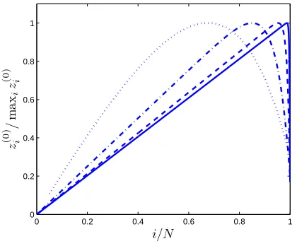
2 ,namely “half-way” between states 0 andN. When it comes to an asymmetric ring network withr >1,however,maxiz(0)i emerges at some stateimwhich is much biased towards stateN as can be seen in Figure 4.1. Numerical experiment indicates that for any fixed r >1, im moves closer to N,as measured by im/N,when N increases. The next two theorems provide asymptotic results concerningim and maxizi(0).
Theorem 4.3. WhenN is sufficiently large,z(0)
i as in (4.1) attains its maximum
at
im=N+ 1−
ln [(N+ 1)(r−1)]
lnr . (4.2)
In addition,
max
i z
(0)
i =
(N+ 1)(r+ 1)
r−1
1 +O
ln(N+ 1)
N+ 1
0 0.2 0.4 0.6 0.8 1 0
0.2 0.4 0.6 0.8 1
i/N
z
(0
)
i
/
ma
xi
z
(0
)
[image:8.612.150.360.114.288.2]i
Fig. 4.1. The dotted, dashdot, dashed, and solid curves representz(0)
i with N-values20,100,
500, and2500, respectively, for the case whenr= 1.2.
Proof. From (4.1),we see that the difference inzi(0) can be written as
z(0)i+1−z (0)
i =
(r+ 1)rN+1−1−(N+ 1)(r−1)ri (r−1)(rN+1−1)
=(r+ 1)
1−r−(N+1)−(N+ 1)(r−1)r−(N+1−i) (r−1)1−r−(N+1) .
Notice that the factor (N+ 1)(r−1)r−(N+1−i) above is increasing ini. Besides,for N large enough,z2(0)−z
(0)
1 >0 andz (0)
N −z
(0)
N−1<0. Consequently,there is a unique maxiz
(0)
i ,which is attained at some 1< i < N.
Continuing,we observe that
zi(0)m+1−z (0) im =
(r+ 1)1−r−(N+1)−(N+ 1)(r−1)r−ln[(N+1)(r−1)]
lnr
(r−1)1−r−(N+1) = −(r+ 1)r−
(N+1)
(r−1)1−r−(N+1) < 0 and,similarly,that
zi(0)m −z (0) im−1=
Finally,substituting (4.2) into (4.1) yields that
zi(0)m =
(N+ 1)(r+ 1)
r−1 −
(r+ 1) ln [(N+ 1)(r−1)] (r−1) lnr −
(r+ 1)rN+1 (r−1)2(rN+1−1) + (N+ 1)(r+ 1)
(r−1)(rN+1−1) = (N+ 1)(r+ 1)
r−1 +O(ln(N+ 1)). This concludes the proof.
It should be mentioned that,in fact,maxizi(0) can be expressed as
max
i z
(0)
i =
(r+ 1)im
r−1 +O(1).
The formulation for maxizi(0) in (4.3),however,turns out to be sufficiently accurate for our purpose.
Theorem 4.4. Let im be given as in (4.2). Then
lim
N→∞
z(0)im
z(0)N = r
r−1. (4.4)
Proof. It is quite straightforward to verify this limit.
We comment that Theorem 4.4 confirms that for N large enough, im is indeed strictly smaller than N because it can be seen from (4.4) thatzi(0)m > z
(0)
N . In addi-tion,this theorem serves as an alternative estimate of maxiz(0)i in terms ofzN(0),i.e.
maxiz (0)
i ≈
rzN(0)
r−1,provided thatN is sufficiently large.
4.2. Modified Markov chain. Next,we investigate the maximum mean first passage time to state 0 on the modified ring network,whose transition matrix Tǫ is formulated as in (2.2).
LetTǫbe the principal submatrix obtained from Tǫ by deleting its first row and column. Similar toz(0),z(ǫ)is determined by
z(ǫ)= (I
−Tǫ)−1e. Note that
where theN×N matrixAis in the form of (3.1) with
c0= 1, c1=ǫ−
µ
r+ 1, and c−1=ǫ−
µr
r+ 1. (4.6)
Obviously,c−1< c1.
Following the methodology of [5,9],we are mainly concerned with the question as to how the small probability ǫ of jumping to non-neighboring states on the ring network affects the maximum mean first passage time to state 0,given that the size of the ring network is large enough. Recall that 0< ǫ≤ N1−1. Especially,c1becomes 0 at ǫ = 1
N+r,which lies in the range
0, 1 N−1
, and thus the results in Section 3 no longer apply. To avoid such singularity,we further assume,without much loss of generality,that
0< ǫ < ǫm= 1
N+r. (4.7)
This additional assumption implies thatc−1< c1<0,as is clear from (4.6).
We continue with several technical lemmas.
Lemma 4.5. Let ci’s be given as in (4.6). Suppose that 0 < ǫ < ǫm. Then the
discriminant as quoted in (3.2) can be written as
δ=(r+ 1)
2−4 [1−(N+r)ǫ] [r−(N r+ 1)ǫ]
(r+ 1)2 . (4.8)
In addition, we have that 0< δ <1 and thatδ is increasing inǫ.
Proof. Note that (N + 1)ǫ < 2 whenever ǫ < ǫm. It can be readily verified by (4.6) that
δ= (N+ 1)ǫ[2−(N+ 1)ǫ] +µ
2(r
−1)2 (r+ 1)2 >0.
This formula forδreduces to (4.8) by combining withµ= 1−(N−1)ǫ.
The fact that δ < 1 can be seen from [1−(N+r)ǫ] [r−(N r+ 1)ǫ] > 0. To justify thatδ is increasing inǫ,we observe that from (4.8),
dδ
dǫ =
4r2+ 2N r+ 1−2(N+r)(N r+ 1)ǫ
(r+ 1)2 .
Since
r2+ 2N r+ 1
2(N+r)(N r+ 1)−ǫm=
r2−1
it follows that dδ
dǫ >0 for any 0< ǫ < ǫm.
Lemma 4.6. For the matrix A as defined in (3.1) with ci’s as given by (4.6),
assuming that 0< ǫ < ǫm, equation (3.3) has two distinct real roots
x1=
(r+ 1)1−√δ
2 [1−(N+r)ǫ] (4.9)
and
x2=
(r+ 1)1 +√δ
2 [1−(N+r)ǫ] (4.10)
such that 0 < x1 < 1, x2 > r, and x1x2 > 1. Furthermore, limǫ→0+x1 = 1, limǫ→0+x2=r,lim
ǫ→ǫ−mx1= r−1
N+r, and limǫ→ǫ−mx2=∞.
Proof. The derivation of (4.9) and (4.10) is straightforward.
It is obvious thatx1>0. On the other hand,we have that
x1=
r+ 1−(r+ 1)2−4 [1−(N+r)ǫ] [r−(N r+ 1)ǫ]
2 [1−(N+r)ǫ] .
Notice that
r+ 1−2 [1−(N+r)ǫ]2−(r+ 1)2−4 [1−(N+r)ǫ] [r−(N r+ 1)ǫ]
=−4(N+ 1)(r+ 1) [1−(N+r)ǫ]ǫ <0,
which implies thatx1<1. The claim that x2> rcan be shown in a similar fashion. In addition,x1x2= c−1
c1 >1 sincec−1< c1<0.
The limits of x1 and x2 while ǫ is pushed towards 0 or ǫm can all be verified directly.
Before proceeding,it should be mentioned that there is an interplay between ǫ
and N,assuming that r is given. In particular,for any specified ǫ, N can not be arbitrarily large due to the restriction,following (4.7),that
N < 1
ǫ −r. (4.11)
We are now ready to return to (4.5). Due to this rank-one update relationship betweenI−TǫandA,it is known [5] that
z(ǫ)= A−1e
1−ǫeTA−1e. (4.12)
By formula (4.12) as well as Lemmas 3.3 and 4.6,it follows:
Theorem 4.7. For the homogeneous ergodic Markov chain with transition matrix
(2.2), the mean first passage time from statei to state 0 is in the form
zi(ǫ)=
A−1e
i
1−ǫeTA−1e, (4.13)
where
A−1e
i =
(x1+x2)x2N+1−xN1+1−xi1xN2+1+xN1+1xi2−xi2+xi1
(xN2+1−x1N+1)(1−x1)(x2−1)
, (4.14)
withx1 andx2 being given by (4.9) and (4.10), respectively.
Proof. The conclusion is immediate. Note thatc1=−x1+1x2.
0 0.2 0.4 0.6 0.8 1
0 0.2 0.4 0.6 0.8 1
i/N
z
(
ǫ
)
i
/
ma
xi
z
(
ǫ
)
[image:12.612.113.445.230.554.2]i
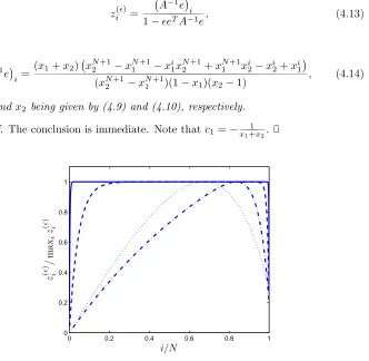
Fig. 4.2. The dotted, dashdot, dashed, and solid curves representz(ǫ)
i withN-values20,100,
500, and2500, respectively, for the case whenǫ= 1×10⁻⁵ andr= 1.2.
Numerical experiments suggest that whenǫis small but prescribed,and whenN
is large enough,unlike maxiz (0)
i ,maxiz
(ǫ)
N. We recall that according to Lemma 3.4,asǫapproaches 0, zi(0) andzi(ǫ)become identical. It should be noted,however,that the test result in Figure 4.2 does not contradict that in Figure 4.1 since the value of ǫ here is fixed,rather than being pushed towards 0.
Using Theorem 4.7,we can establish as follows two asymptotic results concerning
imand maxizi(ǫ).
Theorem 4.8. For any sufficiently small 0 < ǫ < ǫm, when N is sufficiently
large, z(iǫ) attains its maximum at
im=
(N+ 1) lnx2
lnx2
x1
, (4.15)
which satisfies that im> N+12 . Furthermore,
max
i z
(ǫ)
i =
N+ 1
√
δ +O
maxx
N+1
2 1 , x−2N
, (4.16)
whereδ is given as in (4.8).
Proof. First of all,it is clear from (4.13) thatzi(ǫ)is maximized at someiwhenever so isA−1e
i. As a result,it suffices to consider
A−1e
i in order to estimateim. By (4.14),the difference inA−1e
i can be expressed as
A−1e
i+1−
A−1e
i
=(x1+x2)
xi
1(1−x1)
1−x−(N+1) 2
−xi
2(x2−1)1−xN1+1
x−(N+1)
2
1−xN1+1x− (N+1) 2
(1−x1)(x2−1)
.
According to Lemma 4.6,0 < x1 < 1 and x2 > r,leading to the observation that the term xi
1(1−x1)
1−x−(N+1) 2
is decreasing in i,while the term xi 2(x2− 1)1−xN+1
1
x−(N+1)
2 is increasing in i. Besides,for N large enough,
A−1e
2−
A−1e
1 > 0 and
A−1e
N −
A−1e
N−1 < 0. Consequently,there is a unique maxizi(ǫ),which is attained at some 1< i < N.
Continuing,withimas in (4.15),we estimate
A−1e
im+1−
A−1e
im for large
N:
A−1e
im+1−
A−1e
im =
(x1+x2)xi1m
1−xN1+1x− (N+1) 2
(1−x1)(x2−1)
(1−x1)1−x−(N+1) 2 − x 2 x1
(N+1) lnx2 ln(xx21)
(x2−1)1−xN1+1
x−(N+1)
2
≈ (x1+x2)x
im
sincex1+x2= 1−(rN+1+r)ǫ>2. Similarly,we find that
A−1e
im−
A−1e
im−1≈
(x1+x2)xi1m
1 + x1
x2
(1−x1)(x2−1)
>0.
Hence (4.15) is valid.
In addition,again by Lemma 4.6,x1x2 >1,which yields thatim> N2+1. This can be justified by considering 2 lnx2= ln
x2
x1
x1x2
>lnx2
x1
.
Now,using (4.14),we obtain that
A−1e
im =
(x1+x2)
1−xN1+1x− (N+1)
2 −xi
m 1
2−xN1+1−x− (N+1) 2
1−xN1+1x− (N+1) 2
(1−x1)(x2−1) = x1+x2
(1−x1)(x2−1)
+Ox
N+1
2 1
and that
eTA−1e= x1+x2
1−xN1+1x−(N+1) 2
(1−x1)(x2−1)
N1−xN1+1x−
(N+1) 2
−
(x1−xN1+1)
1−x−(N+1) 2
1−x1 −
(1−xN+1 1 )
1−x−N 2
x2−1
= x1+x2 (1−x1)(x2−1)
N−1x1
−x1 − 1
x2−1
+Omax xN1+1, x−2N !
.
Thus,we arrive at the following:
max
i z
(ǫ)
i =
(x1+x2)(1−x1)(x2−1) (1−x1)2(x
2−1)2−ǫ(x1+x2) [N(1−x1)(x2−1)−x1(x2−1)−(1−x1)] +Omaxx
N+1
2 1 , x−2N
. (4.17)
¿From (4.9) and (4.10),it is a matter of direct calculation to verify that
(1−x1)(x2−1) =
(N+ 1)(r+ 1)ǫ
1−(N+r)ǫ .
Also note that,as mentioned earlier in the proof,x1+x2= 1 r+1
−(N+r)ǫ. These reduc-tions,together with (4.9),(4.10),and (4.17),finally yield (4.16).
We mention that from the foregoing proof,it is quite clear that in fact for anyim in the form ofim= (N+ 1)γ,where 0< γ <1 is fixed,
A−1e
im+1−
A−1e
0 1 2 3 4 5 6 7 8
x 10−4
200 300 400 500 600 700 800 900 1000 1100 1200
ǫ
ma
xi
z
(
ǫ
)
i
0 0.5 1 1.5 2 2.5 3 3.5
x 10−4
0 1000 2000 3000 4000 5000 6000
ǫ
ma
xi
z
(
ǫ
)
[image:15.612.52.460.79.267.2]i
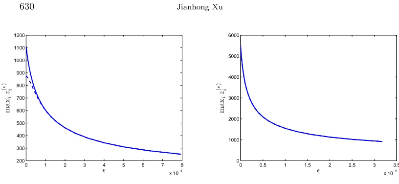
Fig. 4.3.The solid and dashed curves represent the estimate ofmaxiz( ǫ)
i as provided by (4.16)
and the exactmaxiz(
ǫ)
i , respectively. The graph on the left illustrates the case whenN = 100and
r= 1.2, whereas the graph on the right illustrates the case when N = 500 andr= 1.2. For each
case, the smallestǫvalue is determined by10−8/N2.
The formulation of error terms in the preceding proof is based on the observation that 0 < x1 < 1 and x2 > r. Especially,when N is extremely large,i.e. when
ǫ ≈ 1
N+r by (4.11),we see from (4.9) thatx1 ≈ r−1
N+r,which is far smaller than 1. This also implies thatx2is far greater thanrsincex1x2>1. Thus,the error terms in the proof,including the one as in (4.16),are negligible whenN becomes sufficiently large.
The accuracy of the estimate,without the error term,in formula (4.16) is con-firmed by numerical experiment as well. Two such examples are shown in Figure 4.3, where the N-values are indeed quite moderate in light of the ǫ-value. Note that in the graph on the right,the difference between the two curves is barely discernible. Numerical results also evidence that the largerN is,the closer the approximation in (4.16) tends to be towards the actual maxizi(ǫ).
Theorem 4.9. Set ζ(ǫ)= N√+1
δ , whereδ is formulated as in (4.8). Then
lim ǫ→0+ζ
(ǫ)= (N+ 1)(r+ 1)
r−1 ,
i.e.
lim ǫ→0+ζ
(ǫ)
≈max
i z
(0) i ,
provided thatN is sufficiently large. Moreover,ζ(ǫ)is decreasing inǫfor any0< ǫ <
Proof. The claim regarding limǫ→0ζ(ǫ) follows immediately by referring to (4.3) and (4.16). In addition,the monotonicity of ζ(ǫ) is a direct consequence of Lemma 4.5.
Before concluding this section,we comment that the estimates as in (4.3) and (4.16) hinge upon the fact thatr > 1. This means that asr approaches 1,they do not reduce to the corresponding results for the symmetric ring network as can be found in [5]. However,for any fixedr >1,they produce good approximations for the current asymmetric case,provided thatN is sufficiently large.
5. Transient behavior of the Markov chain.
5.1. Reduction ratio. Following [5,9],we define the reduction ratio ρin the maximum mean first passage time to be
ρ= maxiz
(ǫ) i maxizi(0)
. (5.1)
The question that we are concerned with is howρresponds to changes inǫ,the prob-ability of jumping to non-neighboring states,and inr,the ratio of asymmetry,with the assumption that N is sufficiently large. In particular,as in [5,9],an important issue is whether ρundergoes a considerable drop asǫincreases. The development in the preceding section allows us to derive asymptotic results regarding the effects of varyingǫandron the behavior ofρ.
According to Theorems 4.3,4.8,and 4.9,we obtain the following useful result on the reduction ratioρ:
Theorem 5.1. For any sufficiently small 0 < ǫ < ǫm, when N is sufficiently
large, the reduction ratio in (5.1) can be expressed as
ρ=ρ+O
ln(N+ 1)
N+ 1
, (5.2)
where
ρ= r−1
(r+ 1)2−4 [1−(N+r)ǫ] [r−(N r+ 1)ǫ]. (5.3) In addition, we have that limǫ→0+ρ= 1and that ρis decreasing in ǫ.
Theorem 5.2. Let 0 < ǫ < ǫm be sufficiently small. If N is sufficiently large,
then the best reduction ratioρb can be formulated as
ρb=
r−1
r+ 1. (5.4)
Proof. The conclusion follows immediately from (5.3). We point out that estimate (5.4) can be derived in an alternative way. Recall that by Theorem 4.6,limǫ
→ǫ−
mx1=
r−1
N+rand limǫ→ǫ−mx2=∞. On the other hand,we see from (4.17) that,withx
2 2being a dominant factor asǫ is nearǫm,
max
i z
(ǫ)
i ≈
1−x1
(1−x1)2−N(1−x1)ǫ+x 1ǫ
,
which further reduces to a value of N+ 1 as ǫ approaches ǫm. This limit,together with (4.3),lead to (5.4).
Theorem 5.2 reveals the connection between ρb and r. Specifically,when r is close to 1, ρb can be extremely small; as r increases,however,so does ρb,thus less significant the drop in ρis expected to be. A special case of much interest is stated below.
Theorem 5.3. Suppose that 0 < ǫ < ǫm is sufficiently small and that N is
sufficiently large. Then the best reduction ratio ρb ≥1/2 when r≥3. Furthermore, ρb≈1for r large enough.
It is demonstrated in [5] that for a symmetric ring network, ρ ≤ 1/2 so long
as ǫ 32
(N+1)3,meaning that a substantial drop in ρ can always be achieved as ǫ increases. In contrast to this,we see from Theorem 5.3 the rather striking impact of asymmetry on the transient behavior of the ring network: No significant reduction in
ρcan be attained on a large-scale ring network with ratio of asymmetryr≥3.
5.2. Examples. With the estimate in (5.2),we are now in a position to explore numerically the transient behavior of the ring network relative to changes inǫandr.
Following [5,9],we consider that ǫ = k/Nα, where the parameters k > 0 and
α >1. We choosek-values in the rangeNα×10−8< k < Nαǫ
m based on (4.7). We mention that in all numerical trials,the reduction ratioρis computed from formula (5.2) unless stated otherwise.
The role of parameter α is considered in [5,9]. The results in [9] apply to the case whenα= 3,while those in [5] apply to the case whenα >1. Intuitively,varying
10−4 10−2 100 102 0
0.2 0.4 0.6 0.8 1
k
[image:18.612.148.358.114.286.2]ρ
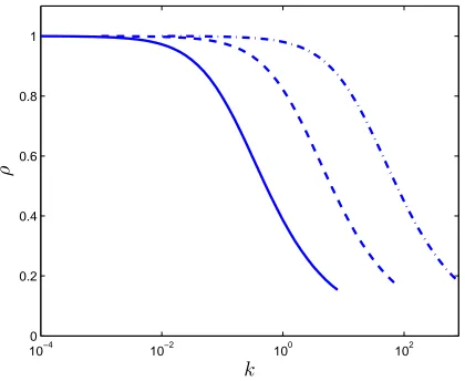
Fig. 5.1.The solid, dashed, and dashdot curves represent the reduction ratioρforα= 1.6,2,
and2.4, respectively. For each case,N andrare fixed atN= 500 andr= 1.2.
100−3 10−2 10−1 100 101
0.2 0.4 0.6 0.8 1
k
ρ
100 101 102 103
0 0.2 0.4 0.6 0.8 1
k
[image:18.612.64.461.344.494.2]ρ
Fig. 5.2. The solid, dashed, and dashdot curves represent the reduction ratioρfor r= 1.2,
1.6, and2, respectively. The graph on the left shows the case whenN= 500andα= 2, whereas the
graph on the right shows the case whenN= 12500andα= 2.
illustrated in Figure 5.1. Notice that the curves in this figure are in fact on different
ǫ-axes.
at thisǫ-value,p= 0.4488 andq= 0.5386 by (2.3),manifesting that the ring network remains to be dominated by asymmetric processes among its neighboring vertices.
Next,we display in Figure 5.2 the effect of varying the ratio of asymmetry ron the reduction ratio ρ. The first observation is that with the growth ofr,the graph ofρ shifts towards the right,verifying that the reduction in ρgradually diminishes. The second observation is that asrgoes up,the maximum drop inρbecomes smaller, confirming the prediction as in Theorem 5.2. WhenN is large enough,as illustrated in the graph on the right,the best reduction ratios forr= 1.2,1.6,and 2 move closer to their estimates from (5.4),namely 0.0909,0.2308,and 0.3333,respectively.
10−3 10−2 10−1 100 101 102 0
0.2 0.4 0.6 0.8 1
k
[image:19.612.149.356.248.421.2]ρ
Fig. 5.3.The solid curve represents the reduction ratioρas in (5.2) for the case whenN= 500,
α= 2, andr= 3. Note that in this example, ǫgoes beyond the range (0, ǫm). The dashed curve
represents the actual reduction ratio as in (5.1) for the sameN,α, andr.
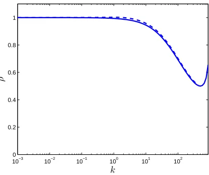
Finally,Figure 5.3 provides an example for the case whenr= 3. There is approx-imately a 50% decrease inρas ǫis nearǫm,which is again consistent with Theorem 5.2. It is interesting to observe in Figure 5.3 that asǫ passes beyondǫm, ρactually starts to bounce back. This indicates in a different perspective,besides consideration of avoiding singularity,that it is indeed reasonable to restrict thatǫ < ǫm. As a com-parison,we also plot in the same figure the exact reduction ratio as obtained from (4.1),(4.13),and (5.1). Clearly,the estimated reduction ratio conforms well,even for
ǫ≥ǫm,to the exact reduction ratio.
Markov chains. In addition,we provide numerical examples to illustrate the conclu-sions.
It is quite interesting to notice that the ratio of asymmetryrplays an important role in determining the transient behavior of the ring network,as measured by the reduction ratio ρ. Specifically,a significant decrease in ρ can be reached when r is close to 1; asrmoves away from 1,however,the decrease inρstarts to diminish. This discovery may shed light on real-world networks where asymmetric interaction takes place,such as those with unbalanced chemical reaction fluxes,traffic flows,energy transfer rates,and bandwidths. Albeit simplistic and crude,the Markov chain model may well address some fundamental issues in applications.
Finally,it should be pointed out that our results are developed within the frame-work of the Markov chain model which is associated with the underlying weighted digraph. It is an intriguing,and important,question as to how these results may be interpreted in the context of the small-world phenomenon on the ring network. Seeking for the answer to this question is a part of our ongoing research.
Acknowledgment. The author is grateful to an anonymous reviewer for con-structive comments on improving the presentation of the results in this paper.
REFERENCES
[1] E.Almaas, B.Kov´acs, T.Vicsek, Z.N.Oltvai, and A.-L.Barab´asi.Global organization of metabolic fluxes in the bacterium Escherichia Coli. Nature, 427(6977):839–843, 2004. [2] H.Balakrishnan and V.N.Padmanabhan. How network asymmetry affects TCP.IEEE Comm.
Magazine, 39(4):2–9, 2001.
[3] A.Barrat, M.Barth´elemy, R.Pastor-Satorras, and A.Vespignani. The architecture of complex weighted networks. Proc. Nat. Acad. Sci., 101(11):3747–3752, 2004.
[4] R.Bellman.Introduction to Matrix Analysis.McGraw-Hill, New York, 1970.
[5] M.Catral, M.Neumann, and J.Xu. Matrix analysis of a Markov chain small-world model.
Linear Algebra Appl., 409:126–146, 2005.
[6] G.E. Cho and C.D. Meyer. Markov chain sensitivity measured by mean first passage times.
Linear Algebra Appl., 316:21–28, 2000.
[7] E.Dietzenbacher.Perturbations and Eigenvectors: Essays.Ph.D.Thesis, University of Gronin-gen, The Netherlands, 1990.
[8] M.Dow. Explicit inverses of Toeplitz and associated matrices.ANZIAM J., 44(E):185–215, 2003.
[9] D.J. Higham. A matrix perturbation view of the small world phenomenon. SIAM J. Matrix
Anal. Appl., 25(4):429–444, 2003.
[10] D.J. Higham. Greedy pathlengths and small world graphs.Linear Algebra Appl., 416:745–758, 2006.
[11] J.G. Kemeny and J.L. Snell. Finite Markov Chains.Van Nostrand, Princeton, New Jersey, 1960.
[13] M.E.J. Newman. The structure and function of complex networks. SIAM Rev., 45(2):167–256, 2003.
[14] M.E.J. Newman, C. Moore, and D.J. Watts. Mean-field solution of the small-world network model. Phys. Rev. Lett., 84:3201–3204, 2000.