Crossover Collision of Scroll Wave Filaments
Bernold Fiedler and Rolf M. Mantel
Received: December 20, 1999 Revised: December 19, 2000 Communicated by Alfred K. Louis
Abstract. Scroll waves are three-dimensional stacks of rotating spi-ral waves, with spispi-ral tips aligned along filament curves. Such spatio-temporal patterns arise, for example, in reaction diffusion systems of excitable media type.
We introduce and explore the crossover collision as the only generic possibility for scroll wave filaments to change their topological knot or linking structure. Our analysis is based on elementary singularity theory, Thom transversality, and abackwards uniqueness property of reaction diffusion systems.
All phenomena are illustrated numerically by six mpeg movies down-loadable at
http://www.mathematik.uni-bielefeld.de/documenta/vol-05/21.html and, in the printed version, with six snapshots from each sequence.
1991 Mathematics Subject Classification: 35B05, 35B30, 35K40, 35K55, 35K57, 37C20
Keywords and Phrases: Parabolic systems, scroll wave patterns, scroll wave filaments, spirals, excitable media, crossover collision, singularity theory, Thom transversality, backwards uniqueness, video.
1 Introduction
Spatio-temporal scroll wave patterns have been observed both experimentally and in numerical simulations of excitable media in three space dimensions. See for example [36, 25, 20] and the references there. Typical experimental settings are the Belousov-Zhabotinsky reactions and its many variants.
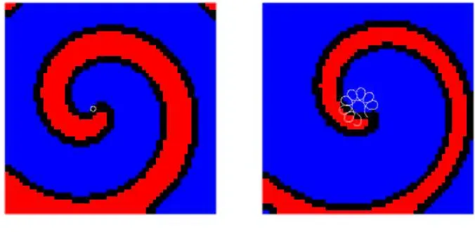
Figure 1: Spiral wave patterns (model see section 6). Shown on the left is a rigidly rotating spiral wave with parameters as in section 6, on the right is a meandering spiral wave, with parametera= 0.65 instead ofa= 0.8. For color coding see section 7.
see [34], 1946. Meandering tip motions are also observed; see for example [35, 38, 5, 4] and the references there. There is some ambiguity in the definition of the tip of a spiral. It is an admissible definition in the sense of [13, sec.4], to associate tip positions (x1, x2)∈R2at timet≥0 with the location of zeros of
two components (u1, u2) of the solution describing the state of the system:
u= (u1, u2)(t, x1, x2) = 0.
(1.1)
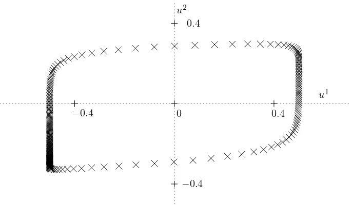
In a typical excitable medium the values of (u1, u2) trace out a cycle as shown
in figure 2, along x-circles around the spiral tip. In a singular perturbation setting, steep wave fronts are observed along these x-circles. Only near the spiral tip, these u-cycles shrink rapidly to the tip-valueu= 0.
This scenario, among other observations, motivated Winfree to attempt a phe-nomenological description in terms of states ϕ=u/|u| ∈ S1, for (almost) all
x∈R2, with remaining singularities of ϕat the tip positions. In the present paper, we return to a reaction diffusion setting for u=u(t, x)∈ R2, keeping
in mind that the set u(t, x) = 0 is particularly visible, distinguished, and de-scriptively important – not as an “organizing center”which causes the global dynamics to follow its pace, but rather as a highly visible indicator of the global dynamics. In fact, defining tip positions by other nonzero levels (t, x)≡ const., inside the cycle of figure 2, works just as well, and only reflects some of the ambiguity in the notion of “tip position”, as was mentioned above. With all our results below holding true, independently of such a shift of u-values, we proceed to work withu(t, x) = 0 as a definition of tip position.
0.4
−0.4
0.4 −0.4
u1
u2
0
Figure 2: A cycle of values (u1, u2)(t, x0) through a time-periodic wave front at a suitably fixed position x0 in an excitable medium (see section 6). Polar coordinates define a phaseϕ∈S1along the dotted cycle.
as stacks of spiral waves with their tips aligned along a one-dimensional curve called the tip filament. As in the planar case, the tip filament may move around in R3, and the associated sectional spirals may continuously change their shapes and their mutual phase relations with time. Denoting by (u1, u2)
two components of the solutions of the associated reaction diffusion systems, again, we can consider filamentsϕtas given by the zero sets
u= (u1, u2)(t, x1, x2, x3) = 0.
(1.2)
We use two components here because the local dynamics of excitable media are essentially two-dimensional. More precisely, for each fixed time t >0 the filamentsϕt describe the zerosx∈R3 of the solution profile
x7→u(t, x). (1.3)
In other words, the filamentϕtis the zero level set of the solution profileu(t,·)
at time t.
Suppose zero is a regular value ofu(t,·), that is, thex-Jacobianux(t,·) possesses
maximal rank 2 at any zero ofu. Then the filamentsϕt consist of embedded
curves inR3, by the implicit function theorem. Moreover the filaments depend as smoothly ontas smoothness of the solutionupermits.
Figure 3: A scroll wave and its filament. The band is tangential to the wave front at the filament.
b.) t=t0 c.) t > t0
a.) t < t0
Figure 4: Crossover collision of oriented filaments at timet=t0
analyze the simplest possible case, we assume
u(t0, x0) = 0,
co-rank ux(t0, x0) = 1.
(1.4)
LetPdenote a rank one projection along rangeux(t0, x0) onto any complement
of that range. Let E = ker ux(t0, x0) denote the two-dimensional null space
of the 2×3 Jacobean matrix ux. We assume the following non-degeneracy
conditions for the time-derivativeut and the Hessianuxx, restricted toE:
P ut(t0, x0) 6= 0, and
P uxx(t0, x0)|E is strictly indefinite.
(1.5)
is given by
In figure 4 we observe the associated crossover collision of filaments in pro-jection onto the null space E: at t = t0 two filaments collide, and then
re-connect. Note that after collision the two filaments do not reconnect as be-fore, re-establishing the previous filaments. Instead, they cross over, forming bridges between originally distinct filaments. Figure 4 describes the universal unfolding, by the time “parameter”t, of a standard transcritical bifurcation in x-space. In fact, supposeu(t, x) satisfies assumptions (1.4), (1.5). Then there exists a local diffeomorphism
τ = τ(t) ξ = ξ(t, x) (1.7)
mapping (t0, x0) to τ0 = t0, ξ0 = 0, such that the original zero set
trans-forms to that of example (1.6), rewritten in (τ, ξ)-coordinates. This follows from Lyapunov-Schmidt reduction and elementary singularity theory; see for example [15].
In an early survey, Tyson and Strogatz [31] hinted at topologically consistent changes of the connectivity of oriented tip filaments, as a theoretical possibility. The point of the present paper is to identify specific singularities, in the sense of singularity theory, which achieve such changes and which, in addition, are generic with respect to the initial conditions of general reaction diffusion sys-tems. Genericity refers to topologically large sets. These sets contain countable intersections of open dense sets, and are dense. We caution our PDE readers here that we are not addressing issues like loss of regularity (smoothness) or development of singularities in a blow-up sense. Genericity is based on pertur-bations of only the initial conditions. We do not require any perturpertur-bations of the underlying partial differential equations themselves.
We consider it a fundamental idea to study solutions u(t, x) of partial differ-ential equations, qualitatively, by investigating the singularities of their level sets – possibly for all, or at least for generic initial conditions. Such an idea is already present in work by Schaeffer, [27], and more recently by Damon, [7], [8], [9] and the references there. In view of example (2.12) for linear scalar parabolic equations in one space dimension below, the first relevant example can even be attributed to Sturm [28], 1836. For present day relevance of Sturm’s observations, once motivated by Sturm-Liouville theory, see also [3], [12], [23]. The work by Schaeffer addresses level sets of strictly convex scalar hyperbolic conservation laws in one space dimension. His analysis is based on the vari-ational formulation due to Lax: for almost every (t, x) the solution u(t, x) appears as the pointwise minimizer of a given function, which involves the initial conditionsu0(x) explicitly. The backwards uniqueness problem, a
Damon’s work is motivated by Gaussian blurring and by applications of the linear heat equation to image processing, but applies to a large class of differ-ential operators. Unfortunately, the partial differdiffer-ential equations are viewed as purely local constraints on thek-jet of “solutions”. Neither initial nor boundary conditions are imposed on these “solutions”. Genericity is understood purely in the space of smooth such “solutions”. The important nonlocal PDE issue of genericity in terms of initial conditions, as addressed in our present paper, has not been resolved by Damon’s approach.
In contrast to these abstract results, strongly in the spirit of pure singularity theory, our motivation is the global qualitative dynamics of reaction diffusion systems. In particular, we do require our solutions u = u(t, x) to not only satisfy the underlying partial differential equations near (t0, x0) but also the
respective initial and boundary conditions. For a technically detailed statement see our main result, theorem 2.1 below. As a consequence, the crossover of filaments just described is the one and only non-destructive collision of filaments possible – for a generic set of initial conditions. See theorem 2.2.
The remaining sections are organized as follows. Preparing for the proof of theorem 2.1, we provide an abstract jet perturbation lemma in section 3 which is based on backwards uniqueness results for linear, non-autonomous parabolic systems. In section 4, we prove theorem 2.1 using Thom’s jet transversality theorem. Moreover we present a generalization to the vector caseu∈Rm, m≥ 2,in corollary 4.2. Theorem 2.2 is proved in section 5. Section 6 summarizes a fast numerical method, due to [11, 22], for time integration of a specific excitable medium with steep fronts in three space dimensions. In section 7 we adapt this method to compute filaments and their associated local isochrone phase bands. We conclude with numerical examples illustrating crossover collisions in autonomous and periodically forced reaction diffusion systems, including the unlinking of linked twisted scroll rings and the unknotting of a trefoil torus knot filament; see section 8.
Acknowledgment. Both authors are grateful to the Institute of Mathematics and its Applications (IMA), Minneapolis, Minnesota. The main part of this work was completed there during a PostDoc stay of the second author and several visits of the first author as senior visiting scientist during the special year ”Emerging Applications of Dynamical Systems”, 1997/98. We are indebted to Jim Damon for helpful discussions, and to the referee for additional references. We thank Martin Rumpf and Peter Serocka for help with visualization. Support by the Deutsche Forschungsgemeinschaft is also gratefully acknowledged.
2 Main Results
For a technical setting we consider semilinear parabolic systems
ui
t= divx(di(t, x)∇xui) +fi(t, x, u,∇xu)
(2.1)
throughout the present paper. Here u = (u1, . . . , um) ∈ Rm, x =
posi-tive definite diffusion matricesdi. The bounded open domain Ω is assumed to
have smooth boundary. Inhomogeneous mixed linear boundary conditions
αi(x)ui(t, x) +βi(x)∂νui(t, x) =γ(x)
(2.2)
with smooth data andαi, βi ≥0, α2i +β2i ≡1 are imposed. Periodic
bound-ary conditions are also admissible, as well as uniformly parabolic semilinear equations on compact manifolds with smooth boundaries, if any.
The solutions
u=u(t, x;u0)
(2.3)
of (2.1), (2.2) with initial condition
u(0, x;u0) :=u0(x)
(2.4)
define a local semi-evolution system in the phase space X of profilesu0(·) in
any of the Sobolev spaces Wk′,p
(Ω), k′
> N/p, which satisfy the boundary conditions (2.2); see [16] for a reference. By the smoothing property of the parabolic system, solutions are in fact smooth in their maximal open intervals of existencet∈(0, t+(u0)) and depend smoothly onu0∈X, both when viewed
pointwise and when viewed asx-profilesu(t,·;u0)∈X.
To address the issue of singularitiesu(t0, x0) = 0, in the sense of singularity
the-ory, we consider thejet space Jk
x of Taylor-polynomials inx= (x1, . . . , xN)∈ RN of degree at mostk, with real coefficients and vector valuesu∈Rm.
Defin-ing thek-jetjk
Here and below, we assume thatk′
> k+N/pso that the evaluation
u7→jxku(t0, x0)
(2.7)
becomes a bounded linear map fromX toJk
x, by Sobolev embedding.
On the level ofk-jets, a notion of equivalence is induced by the action of local Ck-diffeomorphismsx7→Φ(x), u7→Ψ(u) fixing the origins ofx∈RN, u∈Rm,
respectively. Indeed, for any polynomial p(x) ∈ Jxk with p(0) = 0, we may
consider the transformed polynomial
jkx(Ψ◦p◦Φ)∈Jxk.
(2.8)
We call the jet (2.8)contact equivalenttojk
By avariety S⊂Rℓ we here mean a finite disjoint union
of embedded submanifolds Sj ⊂Rℓ with strictly decreasing dimensions such
thatSj1∪. . .∪Sj0 is closed for anyj1. We call codimRℓS0 the codimension of the varietyS in Rℓ.
Similarly, by asingularity(in the sense of singularity theory) we mean a variety S ⊂Jk
x in the sense of (2.9), which satisfiesu= 0 and is invariant under any
of the contact equivalences (2.8). Let codimJk
xS denote the codimension of S, viewed as a subvariety of Jk
x. Shifting codimension by N = dimx for
convenience we call
higher. In contrast, the map can be expected to hit singularities S of codi-mension 1 at isolated points t = t0, and for somex0 ∈ RN. Having shifted
codimension by N in (2.10) therefore conveniently allows us to observe that typical profiles of functionsu(t,·) miss singularities of codimension 2 entirely, and encounter such singularities of codimension 1, anywhere in x∈ RN, only at discrete times t.We aim to show that this simple arithmetic also works for PDE solutionsu(t, x) under generic initial conditions.
Since the geometrically simple issue of codimension is overloaded with – some-times conflicting – definitions in singularity theory, we add some examples which illustrate our terminology. First consider the simplest case
S={u= 0} ⊂Jk x.
(2.11)
where u(t,·) : RN → Rm. Then codimS = m−N. For systems ofm = 2
equations inN = 0 space dimensions, that is, for ordinary differential equations in the plane, typical trajectories fail to pass through the origin in finite time: codimS = 2. For N = 1, we can expect the solution curve profileu(t,·) to pass through the origin at certain discrete times t0 and positions x0, because
codimS = 1. For N = 2 we have codimS = 0. We therefore expect isolated zeros to move continuously with time: see our intuitive description of planar spiral waves in section 1 and figure 1. Since codimS = −1 for N = 3, we expect zeros ofu(t0,·) to occur along one-dimensional filaments, even for fixed
t0. This is the case of scroll wave filaments ϕt0 in excitable media.
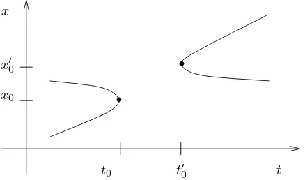
Next we consider a scalar one-dimensional equation, m = N = 1. Multiple zeros are characterized by
S ={u= 0, ux= 0},
x0
x′ 0
x
t t0 t′0
Figure 5: Saddle-node singularities of codimension 1.
a set to which we ascribe codimension 1. Indeed, we can typically expect a pair of zeros to coalesce and disappear as in (t0, x0) of figure 5. The opposite case,
a pair creation of zeros as in (t′ 0, x
′
0), does not occur for scalar nonlinearities
f satisfyingf(t, x,0,0) = 0. This observation, going back essentially to Sturm [28], conveys considerable global consequences for the associated semiflows; see for example [12] and the references there.
Passing to planar 2-systems,m=N= 2, the same saddle-node bifurcations of figure 5 could for example correspond to annihilation and creation of a pair of tips of counter-rotating spirals, respectively.
We conclude our series of motivating examples with the singularity (1.4) of filament collision in systems satisfyingN =m+ 1:
S ={u= 0, co-rankux≥1}.
(2.13)
Note that codimS= 1. For the stratum S0 ofS with lowest codimension we
can assume that the quadratic form P uxx|E is indeed nondegenerate, in the
notation of (1.5). Under the additional transversality assumptionP ut6= 0, the
strictly indefinite case was discussed in section 1. It leads to crossover collisions, which are our main applied motivation here. The strictly definite case, positive or negative, leads to creation/annihilation of small circular filaments. For a numerical realization of the associated scroll ring annihilation we refer to the simulation in figure 8.
After our intermezzo on singularities we now address genericity. We say that a property of solutions u(t, x;u0) of our semilinear parabolic system (2.1) –
(2.4) holds forgeneric initial conditionsu0∈X if it holds for a generic subset
of initial conditions. Here subsets are generic (or residual) if they contain a countable intersection of open dense subsets ofX. Recall that generic subsets and countable intersections of generic subsets are dense in complete metric spacesX, by Baire’s theorem; see [10, ch. 12].
t t′
0
t0
x′ 0
x0
x
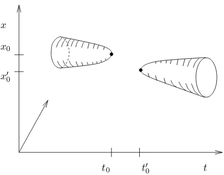
Figure 6: Annihilation (left) and creation (right) of closed filaments
X ⊂Wk′,p
֒→Ck. As before 0≤t < t
+(u0) denotes the maximal interval of
existence. Finally, we recall that a map ρ: V →J between Banach spaces is transverseto a varietyS=S0∪. . .∪Sj0, in symbols:
ρ⊤∩S, (2.14)
ifρ(v)∈Sj implies
Tρ(v)Sj+ rangeDρ(v) =J;
(2.15)
see for example [1, 19].
Theorem 2.1 For some fixedk≥1, consider a finite collection of singularities Si ⊂ Jk
x, each of codimension at least 1. Then the following holds true for
solutions u(t, x)of (2.1) – (2.4) with generic initial conditionsu0∈X.
Singularities Si with
codimSi≥2
(2.16)
are not encountered at any (t0, x0) ∈ (0, t+(u0)) ×Ω. In other words,
jk
xu(t0, x0) ∈ Si for some 0 < t0 < t+(u0), x0 ∈ Ω implies codimSi = 1.
The map
(0, t+(u0))×Ω → Jxk
(t0, x0) 7→ jxku(t0, x0)
(2.17)
is in fact transverse to each of the varietiesSi. In particular, the points(tn 0, xn0)
where the solution u(t, x)encounters singularitiesSiof codimension 1 are
iso-lated in the domain[0, t+(u0))×Ωof existence. Although there can be countably
many singular points(tn
0, xn0)accumulating to the boundary t+(u0)or∂Ω, the
values tn
Theorem 2.2 For some fixedk≥1, consider solutionsu(t, x)of (2.1) – (2.4) with N = 3, m = 2, that is with x ∈ Ω ⊂ R3 and u(t, x) ∈ R2. Then for
generic initial conditions u0∈X the following holds true.
Except for at most countably many timest=tn
0 ∈(0, t+(u0)), the filaments
{x∈Ω|u(t, x) = 0} (2.18)
are curves embedded in Ω, possibly accumulating at the boundary. At each exceptional valuet=tn
0, exactly one of the following occurs at a unique location
xn 0 ∈Ω:
(i) a creation of a closed filament, or
(ii) an annihilation of a closed filament, or
(iii) a crossover collision of filaments.
For cases (i),(ii) see figures 6, 8; for case (iii) see figures 4, 9–13, and (1.4) – (1.6).
3 Jet Perturbation
In this section we prove a perturbation result, lemma 3.1, which is crucial to our proof of theorem 2.1. We work in the technical setting of semilinear parabolic systems (2.1) – (2.4) with associated evolution
u=u(t, x;u0)
(3.1)
on the phase spaceXofWk′,p
(Ω)-profilesu(t,·,;u0) satisfying Robin boundary
conditions (2.2). Let k′
− N
p > k ≥ 1, to ensure the Sobolev embedding
X ֒→Ck(Ω). Let
D:={(t, x, u0)|x∈Ω, u0∈X, 0< t < t+(u0)}
(3.2)
denote the interior of the domain of definition.
Lemma 3.1 The map jk
xu: D → Jxk
(t, x, u0) 7→ jxku(t, x;u0)
(3.3)
is aCκ map, for anyκ. For any(t, x, u
0)∈ D, the derivative
Du0j
k
xu(t, x;u0) : X →Jxk
(3.4)
Proof:
The regularity claim follows from smoothness of the data di, fi, α
i, βi and the
smoothing action of parabolic systems; see for example [16, 26, 29, 14, 21]. To prove surjectivity of the linearization (3.4) with respect to the initial con-dition, we essentially follow [16]. First observe that for any fixed x0 ∈Ω the
linear evaluation map
is bounded, because X ֒→Ck(Ω), and trivially surjective. Moreover, the jet
space Jk
x is finite-dimensional. It is therefore sufficient to show that the
lin-earization
ThenX contains a nonzero element w(t0,·) in theL2-orthogonal complement
of Du0u(t,·;u0)X in X. Consider the associated solution w(t,·) ∈ X of the
for 0≤t≤t0, still with boundary conditions (2.2) but with “initial” condition
w(t0,·) att=t0. We again use the notationfpji for the partial derivative off
j
with respect to ∇ui, here.
Direct calculation shows that scalar products h·,·i between solutionsv(t,·) of the linearization (3.7) and solutionsw(t,·) of its formal adjoint (3.9) inL2(Ω)
are time-independent. Therefore, by construction ofw(t0,·)
for allv0∈X, and hence
w(0,·) = 0. (3.12)
In other words, the backwards parabolic system (3.9) possesses a solutionw(t,·) which starts nonzero att=t0>0 but ends up zero att= 0. This is a
contra-diction to the so-called backwards uniqueness property of parabolic equations. See for example [14], [16] and the references there. By contradiction, we have therefore proved that
closXDu0u(t0,·;u0)X =X,
(3.13)
contrary to our indirect assumption (3.8). This completes the indirect proof of
the perturbation lemma. ⊲⊳
4 Proof of Theorem 2.1
Our proof of theorem 2.1 is based on Thom’s transversality theorem [30, 1]. For convenience we first recall a modest adaptation of the transversality theorem, fixing notation. We use the concept of transversality of a mapρto a varietyS as explained in (2.9), (2.14), (2.15). The proof is based on Sard’s theorem and is not reproduced here.
Theorem 4.1 [Thom transversality] Let X be a Banach space, D ⊆Rℓ×X open and
ρ:D → Rℓ′
(y, u0) 7→ ρ(y, u0)
(4.1)
aCκ-map. LetS⊂Rℓ′
be a variety and assume
ρ⊤∩S, (4.2)
κ >max{0, ℓ−codimRℓ′S}.
(4.3)
Then the set
XS :={u0∈X |ρ(·, u0)S, where defined}
(4.4)
is generic inX (that is: contains a countable intersection of open dense sets).
The point of the theorem is, of course, that in XS transversality to S is
achieved, for fixedu0, by varying onlyy inρ(y, u0). For example,u0∈XS and
codimRℓ′S > ℓimply
ρ(y, u0)6∈S
whenevery is such that (y, u0)∈ D. This follows immediately from condition
(2.15) on transversality. In other words, for generic u0 the image of ρ(·, u0)
misses varieties of sufficiently high codimension.
We now use theorem 4.1 to prove our main result, theorem 2.1. We consider the jet evaluation map
ρ(t, x, u0) :=jxku(t, x;u0)
(4.6)
of the evolutionu(t,·;u0) associated to our parabolic system; see (2.1) – (2.5).
We chooseDto be the (open) domain of definition
D={(t, x, u0)|0< t < t+(u0), x∈Ω, u0∈X}
(4.7)
of the evolution; clearlyy= (t, x)∈RN+1 so that ℓ=N+ 1. For the variety
S we choose, successively, any of the finitely many singularities Si ⊂ Jk x of
theorem (2.1). Their codimensions as subvarieties ofJk x ∼=Rℓ
see (2.10). Note that assumptions (4.2) and (4.3) both hold, independently of the choice of k for the varieties Si ⊆ Jk
x, by lemma 3.1. Claim (2.17) about
transversality of (t0, x0) 7→u(t0, x0;u0) to any singularity Si is now just the
statement of theorem 4.1.
Next, we prove that singularities Si with codimSi≥2 are missed altogether,
for generic initial conditions u0 ∈ X, as was claimed in (2.16). We evaluate
(4.8) to yield
codimJk xS
i =N+ codimSi≥N+ 2> N+ 1 =ℓ
(4.9)
In view of example (4.5), this proves our claim (2.16): generically, only singu-laritiesSi with codimSi= 1 are encountered.
Now we prove that the positions (tn
0, xn0), where singularitiesSiwith codimSi=
1 are encountered, are generically isolated in [0, t+(u0))×Ω. Indeed
assum-ing jk
xu0 6∈ Si, we have tn0 > 0 without loss of generality. Since the
lower-dimensional strataSi
j, j ≥1 of the singularitySiare of (singularity)
codimen-sion≥2, they are missed by solutions entirely, for generic initial conditionsu0.
Therefore
jk
xu(tn0, x0n;u0)∈S0i
(4.10)
only hit the maximal strata, staying away from the closed union of lower-dimensional strata, uniformly in compact subsets of [0, t+(u0))×Ω. Because
theSi
0are finitely many embedded submanifolds of codimensionN+1 inJxkand
because the crossings (4.10) are transverse, the corresponding crossing points (tn
0, xn0) are also isolated in [0, t+(u0))×Ω, as claimed.
It remains to show that the values tn
0 are mutually distinct for generic initial
conditionsu0∈X. To this end we consider the augmented map
˜
ρ: ˜D →Jk x×Jxk
(t, x1, x2, u0)→(jxku(t, x1;u0), jxku(t, x2;u0))
on the open domain
˜
D:={(t, x1, x2, u0)|0< t < t+(u), x1, x2∈Ω, x16=x2, u0∈X}.
(4.12)
To apply Thom’s transversality theorem 4.1, we only need to check the transver-sality assumption (4.2). In fact we show
˜
ρ⊤ {∩ 0} ∈Jk x×Jxk.
(4.13)
This follows, analogously to lemma 3.1, from x1 6= x2 and the fact that the
linearizationDu0u(t0,·;u0) possesses dense range inX; see (3.6) – (3.13). We can therefore apply theorem 4.1 to ˜ρwith respect to the varieties
˜
x×Jxk, these varieties have codimension
codimJk
again. Therefore the times tn
0 where singularities Si can occur are pairwise
distinct for generic initial conditions, completing the proof of theorem 2.1. ⊲⊳
Reviewing the proof of theorem 2.1, which hinges crucially on the transversality statement (3.4) of our jet perturbation lemma 3.1, we state an easy generaliza-tion which is important from an applied viewpoint. Suppose that onlym′
≤m
for some linear rank m′
projection of Rm. Then bu(t, x;u
0) may encounter
certain singularitiesSbi in the spaceJbk
x ofk-jets with values in rangePb.
Corollary 4.2 Under the assumptions of theorem 2.1 and in the above set-ting, theorem 2.1 remains valid, verbatim, for singularitiesSbi⊂Jbk
Therefore the surjectivity property (3.4) of lemma 3.1 remains valid for
Du0jxkub(t, x;u0) : X →Jbk.
(4.19)
Repeating the proof of theorem 4.1, now on the level of u,b Jbk
x,Sbi, proves the
corollary. ⊲⊳
5 Proof of Theorem 2.2
To prove theorem 2.2 we invoke theorem 2.1 forx∈Ω⊂R3, u(t, x)∈R2, and appropriate singularitiesSi⊂Jk
x of singularity codimension 1, in the sense of
(2.10).
We first consider the case that 0 is a regular value ofu(t,·) on Ω, that is
rankux(t0, x0) = 2
(5.1)
is maximal, whenever u(t0, x0) = 0, 0 < t0 < t+(u0), x0 ∈ Ω. Then the
filament
{x∈Ω|u(t0, x) = 0}
(5.2)
is an embedded curve in Ω, as claimed in (2.18). Next consider the case
rankux(t0, x0)≤1.
(5.3)
Let S ⊂Jk=2
x be the set of those 2-jets (u, ux, uxx) ∈Jxk=2 satisfyingu= 0
and rankux= 1. ClearlyS is a singularity in the sense of (2.9), (2.10) and
codimS= 1 (5.4)
as was discussed in example (2.13). We recall that the maximal stratumS0of
S, determining the codimension, is given by the conditions
rankux= 1,
P uxx|E nondegenerate.
(5.5)
HereE := keruxdenotes the kernel andP denotes a projection inR2onto a
complement of the range of the Jacobianux.
In view of example (2.13) and section 1, nondegeneracy ofP uxx|E gives rise to
the three cases (i) - (iii) of corollary 2.2, via theorem 2.1, if only we show that
P ut(t0, x0)6= 0
(5.6)
wheneverj2
xu(t0, x0)∈S.
By theorem 2.1, we have
in J2
and the proof of corollary 2.2 is complete. ⊲⊳
6 Numerical Model and Methods
For our numerical simulations, we use two-variable N = 2 reaction-diffusion equations
∂tu˜1= △u˜1+f(˜u1,u˜2)
∂tu˜2=D△u˜2+g(˜u1,u˜2)
(6.1)
on a square or cube Ω with Neumann boundary conditions. The functions f(˜u1,u˜2) and g(˜u1,u˜2) express the local reaction kinetics of the two variables
˜
u1and ˜u2. The diffusion coefficient for the ˜u1variable has been scaled to unity,
andD is the ratio of diffusion coefficients. For the reaction kinetics we use
f(˜u1,u˜2) =ǫ−1u˜1(1−˜u1)(˜u1−u th(˜u2))
g(˜u1,˜u2) = ˜u1−u˜2,
(6.2)
with uth(˜u2) = (˜u2 +b)/a. This choice differs from traditional
FitzHugh-Nagumo equations, but facilitates fast computer simulations [11]. In non-autonomous simulations, we periodically force the excitability threshold b = b(t) =b0+Acos(ωt). We keep most model parameters fixed ata= 0.8, b0=
0.01, ǫ= 0.02, andD= 0.5.
Without forcing, the medium is strongly excitable, see figure 1. See figure 2 for the dynamics of a wave train. In two space dimensions, the equations generate rigidly rotating spirals with small cores. These spirals are far from the meander instability, and appropriate initial conditions quickly converge to rotating waves. We map the coordinates (˜u1,˜u2) into the (u1, u2)-coordinates
of theorem 2.1 by setting u1 = ˜u1−0.5 and u2 = ˜u2−(a/2−b
0). We have
remarked in the introduction, already, that our results are not effected by such a shift of level sets.
In the autonomous cases we choose a forcing amplitude A= 0, of course. For collision of spirals in two dimensions, we choose A = 0.01, ω = 3.21. For collision of scroll wave filaments in three dimensions, we chooseA= 0.01, ω= 3.92.
and temporal resolutions have to be high, the main computational speedup is achieved by minimizing the number of operations necessary per time step and space point.
Simulations with cellular automata encounter problems due to grid isotropies [17, 32, 33]. The existence of persistent spatial wave fronts impedes algorithms with variable time steps. Due to linearity of the spatial operator, methods with fixed, small time steps are feasible. Moreover, ˜u1 and ˜u2 can be updated in
place away from the wave front.
We use a third-order semi-implicit stepping routine to time step f, combined with explicit Euler time stepping forg and the Laplacian term. In the eval-uation of f and in the diffusion of ˜u1, we take into account that ˜u1 ≈0 in a
large part of the domain, and that f(0,u˜2) = 0. This allows a cheap update
of approximately half of the grid elements and, even with a straightforward finite-difference method, enables simulation on a workstation. The extra effort of an adaptive grid with frequent re-meshing has been avoided.
In three space dimensionsN = 3, we use a 19-point stencil with good numerical properties (isotropic error, mild time-step constraint) for approximating the Laplacian operator. In two dimensions N = 2, we use the analogous 9-point stencil. Neumann boundary conditions are imposed on all boundaries.
For specific simulation runs in this paper, we take 1253grid points. The domain
Ω is chosen sufficiently large, in terms of diffusion length, to exhibit scroll wave collision phenomena. The time step△tis chosen close to maximal: leth denote grid size,σ= 3/8 the stability limit of the Laplacian stencil, and choose △t := 0.784σh2. This results in the following numerical parameters: domain
Ω = −[15,15]3, grid spacing h = 30/124 ≈ 1/4, time step △t = 0.0172086,
giving △t/ǫ = 0.86043. For high-accuracy studies of the collision of scroll waves, we use a higher resolution of Ω = [−10,10]3, h= 20/124≈1/6,△t =
0.00764828, giving△t/ǫ= 0.3882414. Note that△t/ǫ <1 in both cases, which means that the temporal dynamics are well resolved. Further numerical details for the three-dimensional simulations are given in [11].
7 Filament Visualization
After discretization in the cube domain Ω, and time integration, the solution datau(t, x)∈R2are given as valuesu(ti, xi) at time stepsti and at positions
xion a Cartesian lattice. In our two-dimensional examples, figure 1 and
exam-ple 8.2, we show the vector field (˜u1,˜u2) = (u1+ 0.5, u2+ (a/2−b
0), choosing
for each point a color vector in RGB space of (u1,0.73∗(u2)2,1.56∗u2). We
also mark the (past) trace of the tip path in white, to keep track of the move-ments of the spiral tip. In figure 3 and example 8.3, we depict the wave front in x∈Ω as the surface u1= 0.
To determine the filament location, alias the level set
ϕt:={x∈Ω|u1(t, x) =u2(t, x) = 0},
(7.1)
As in section 6, let Q⊆Ω be any of the small discretization cubes. We trian-gulate its faces by bisecting diagonals, denoting the resulting closed triangles byτ. The corners ofτ are vertices ofQ. We orientτ according to the induced orientation of ∂Qby its outward normalν and the right hand rule applied to (τ, ν).
By linear interpolation,u(t, τ)⊂R2 is also an oriented triangle. The filament
ϕtpasses throughτ, on the discretized level, if and only if 0∈u(t, τ). Inverting
the linear approximation u on τ defines an approximation ϕt
ι ∈ τ to ϕt∩τ.
We orient ϕt to leave Q through τ, if the orientation of the triangle u(t, τ)
is positive (”door out”). In the opposite case of negative orientation we say that ϕt enters Q through τ (”door in”). By elementary degree theory, the
numbers of in-doors and of out-doors coincide for any small discretization cube Q. Matching in-doorsϕt
ι and out-doorsϕtι′ in pairs defines a piecewise linear,
oriented approximation to the filament ϕt. For orientations before and after
crossover-collision see figure 4.
Note that here and below, we freely discard certain degenerate, non-generic situations from our discussion which complicate the presentation and tend to confuse the simple issue. In fact, due to homotopy invariance of Brouwer degree, this piecewise linear (PL) method is robust with respect to perturbations of degeneracies like filaments touching a face of the cubeQor repeatedly threading through the same triangleτ.
To indicate the phase near the filamentϕt, we compute a tangential
approxi-mation to the accompanying somewhat arbitrary isochrone
χt:={x∈Ω|u1(t, x)≥0 =u2(t, x)}
(7.2)
as follows. The values (u1, u2)(t, x) = (α,0) with α > 0 define a local half
line in the face triangle x ∈ τ through the filament point ϕt
ι ∈ τ. Together
with a filament point ϕt
ι−1 in another cube face, this half line also defines a
half space which approximates the isochroneχt, locally . We choose a point
˜ ϕt
ι in this half space, a fixed distance from ϕtι and such that the line from
ϕt
ι to ˜ϕtι is orthogonal to the filament line from ϕtι−1 to ϕtι. The sequence
of triangles (ϕt
ι−1,ϕ˜tι−1,ϕ˜tι),(ϕtι−1,ϕ˜tι, ϕtι) then define a triangulated isochrone
band approximatingχtnear the filamentϕt.
In practical computations shown in the next section, we distinguish an absolute front and back of the isochrone band by color, independently of camera angle and position. This difference reflects the absolute orientation of filaments, in-troduced above, which induces an absolute orientation and an absolute normal for the accompanying isochrone χt. The absolute normal of the isochrone χt
also points into the propagation direction of the isochrone, by our choice of orientation.
8 Examples
based on equations (6.1) with the set of nonlinearities and parameters speci-fied there. We use a cube Ω = [−15,15]3 as a spatial domain, together with
Neumann boundary conditions. Only in example 8.4, we use a smaller cube Ω = [−10,10]3.Reflecting the solutions through the boundaries we obtain an
extension to the larger cube 2Ω with periodic boundary conditions. Viewing this system on the flat 3-torusT3, equivalently, eliminates all boundary
con-ditions and avoids the issue of ∂Ω not being smooth. In the paper version, each of the spatio-temporal singularities at (t0, x0) is illustrated by a series of
still shots: t'0, t/t0, t=t0, t't0 and t=tend for the respective run. In
the Internet version, each sequence is replaced by a downloadable animation in MPEG-1 format; see
http://www.math.fu-berlin.de/~Dynamik/
For possible later, updated and revised versions, please contact the authors. Discretization was performed by 1253cubes and a time step of△t= 0.0172086
(△t = 0.00764828 in example 8.4); see section 6. Autonomous cases refer to the forcing amplitude A= 0, whereas A= 0.01 switches on non-autonomous additive forcing.
8.1 Initial Conditions
Prescribing approximate initial conditions for colliding scroll waves in three space dimensions is a somewhat delicate issue. We describe the construction in 8.1.1, 8.1.2 below. We discuss our four examples in sections 8.3-8.6.
8.1.1 Two-dimensional spirals
According to our numerical simulations, planar spiral waves are very robust objects. In fact, sufficiently separated nondegenerate zeroes of the planar “vec-tor field” (u1
0, u20)(x1, x2) of initial conditions typically seemed to converge into
collections of single-armed spiral waves. Their tips were located nearby the prescribed zeroes ofu0.
To prepare for our construction of scroll waves below, we nevertheless construct u0 as a composition of two maps,
u0 = σ◦γ
(8.1)
γ: R2⊇Ω → C (8.2)
(x1, x2) 7→ z
σ: C → R2 (8.3)
z 7→ (u10, u20)
Hereγprescribes the geometric location of the spiral tip and wave fronts. The scaling mapσ is chosen piecewise linear. It adjusts for the appropriate range ofu-values to trace out a wave front cycle in our excitable medium, see fig. 2. Specifically, we choose
near the origin. Further away, we cut off by constants as follows:
In the following, we will sometimes further decomposeσ=σ2◦σ1 where
σ1(z) = (Re(z),Im(z)/4)
(8.6)
is linear and the clampingσ2:R2→R2is the cut-off
(u1, u2)7→(sign(u1) min{|u1|,0.5},sign(u2) min{|u2|,0.4}). (8.7)
For example, this choice of σ, combined with the simplest geometry map γ(x1, x2) = x1 + ix2, results in a spiral wave rotating clockwise around
the origin, with wave front at x1 = 0, x2 < 0, initially, and wave back at
x1= 0, x2>0.
A possible initial condition for a spiral — antispiral pair as in example 8.2 below would be
γ: [−15,15]2 → C
(x1, x2) 7→ |x1| −6 + ix2.
This reflection symmetric initial condition creates a pair of spirals rotating around (±6,0). The spiral at (6,0) rotates clockwise and the symmetric spiral around (−6,0) rotates anti-clockwise.
8.1.2 Three-dimensional scrolls
It is useful to visualize a three-dimensional scroll wave as a stack foliated by two-dimensional slices which contain planar spirals. Initial conditionsu0=σ◦γfor
scroll waves then contain the following ingredients: a mappingγ:R3→Cthat stacks the spirals into the desired three-dimensional geometry, and a scaling σ : C → R2. For planar γ: R2 → C as in (8.2), the scaling σ of (8.3)– (8.7) generates a spiral whose tip is at the origin in R2. Forγ: R3 →C, the
preimage inR3 of the origin under the stacking mapγ will therefore comprise
the filament of the three-dimensional scroll wave. For example, it is easy to find a stacking map γ that gives rise to a single straight scroll wave with vertical filament: γ(x1, x2, x3) :=x1+ ix2. As soon as filaments are required to form
For the generation of more complicated stacking mapsγ, we largely follow the method pioneered by Winfree et al [37, 18, 39]. This approach uses a standard method of embedding an algebraic knot in 3-space [6]. For convenience of our readers, we briefly recall the construction here.
We construct stacking maps γ: R3 → C with prescribed, possibly linked or knotted zero set as a composition
γ=p◦s.
denoting the inverse of the standard stereographic projection from the standard 3- sphereS3
εof radiusεtoR3; see (8.11) below. The map
p: C2→C (8.10)
is a complex polynomial p = p(z1, z2) in two complex variables z1, z2. The
zero set of pdescribes a real, two-dimensional variety V in C2. Consider the intersection ˜ϕofV with the small 3-sphereS3
ε, that is ˜ϕ:=V ∩S3ε. Typically,
ϕ := s−1( ˜ϕ) ⊂ R3, the zero set of γ, will be a one-dimensional curve or a
collection of curves: the desired filament of our scroll wave.
In the simplest case ϕ may be a circle embedded into the 3-sphere S3 ε. If
however zero is a critical point of the polynomialp, then the filamentϕneed not be a topological circle. And even if ˜ϕhappens to be a topological circle, it may be embedded as a knot inS3
ε.
The inverse stereographic map ˜sis given explicitly by
˜
lower hemisphere, points outsideS2
ε to the upper hemisphere ofS3ε.
In our construction (8.8) of the stacking map γ, we now replace the inverse stereographic map ˜sby the embedding
s(x1, x2, x3)∼=c
the embedded paraboloid s(R3) can in fact be modified outside s(Ω) without changing the filaments in Ω. We modify ssuch that closs(R3) closes up to a diffeomorphically embedded 3-shereSdiffeotopic toS3 inC2\ {0},by a family
sϑ of embeddings 0≤ϑ≤1. Moreover, we will choosep=p(z1, z2) such that
z1 = z2 = 0 is the only critical point of p in C2. If the embedding sϑ(R3)
remains transverse to p−1(0) in C2\ {0} throughout the diffeotopy, then the
varietyp−1(0) is an embedded real surface in C2, outsidez= 0. The filament
˜
ϕ =s(ϕ) =p−1(0)∩s(Ω) is diffeotopic to some components of p−1(0)∩S3 ε,
which in turn are described classically in algebraic geometry.
The same remarks apply, slightly more generally, if we replacesby a compo-sition
s◦ℓ (8.13)
whereℓ denotes a nondegenerate affine transformation inR3.
In summary, we generate our initial conditions by applying the following com-position of mappings:
u0=σ◦γ= (σ2◦σ1)◦(p◦s).
(8.14)
Here the scalingσis given by (8.5)–(8.7). The modified stereographic projec-tions is given by (8.12) with ℓ = id, except in example 8.5, and with appro-priate scaling constantc. The polynomialpis chosen according to the desired topology of the filament.
The initial conditions thus created do not necessarily respect the boundary con-ditions; however any intersection of a filament with the boundary is transverse. Anyways, such intersections only occur in example 8.4. Neumann boundary conditions can be enforced artificially, by standard implementation, without introducing additional filaments.
8.2 Two-dimensional spiral pair annihilation
As a preparation to visualizing the three-dimensional behavior, we begin with the collision of a pair of counter-rotating planar spirals. We use a domain Ω = [−15,15]2 and discretize with 1252 grid points, resulting in the same
spatial and temporal resolution as with our three-dimensional experiments. In the movie and pictures, we show the subdomain [−15,15]×[−11.25,11.25] to get the 3:4 size ratio typical for video.
For initial conditions, we take the fully developed rigidly rotating spiral of figure 1 with origin at (−6,0), for the half-planex1≤0, and reflect at the
ver-tical x2-axis. Near-resonant periodic forcing with an amplitude A= 0.01 and
t= 0 t= 19.60
t= 31.77 t= 35.08
t= 37.67 t= 38.46
Figure 7: Interaction and collision of a pair of spiral waves in the plane. MPEG-Movie [26.4MB,gzipped]
length). During the interaction time of the spiral tips, the u2 gradients are
much shallower than at other times. This can be seen by the fact that the bright red part of the wave front is further away from the tip location. The spirals then wander along the vertical axis, the excited center getting smaller with every revolution. Finally the center is too small to sustain exci-tation (t0 = 39.825) and disappears; the spirals annihilate. The purely local
interaction between the spiral tips shortly before collision from timet∗
= 19.2 up to the extinction att0 = 39.825, x0= (0,1.4) is clearly visible from the tip
paths.
In view of theorem 2.1, this annihilation illustrates the left saddle-node singu-larity of fig. 5 for dimu= dimx= 2.
8.3 Scroll ring annihilation
Our first three-dimensional example shows the disappearance of a closed cir-cular filament as described, from an abstract singularity theory point of view, in theorem 2.2,(ii), and as illustrated in figure 6. The example is autonomous, A = 0. Viewed in a vertical planar slice through the center, the dynamics is reminiscent of the two-dimensional spiral pair annihilation 8.2. Instead of pe-riodic forcing, this time, the curvature of the three-dimensional filament seems to be responsible for the filament contraction and annihilation [24].
The simplest initial conditions to create a scroll ring would be via the poly-nomial p(z1, z2) =z2, resulting in the vertical axis ˜s(Rez2) =x3 = 0 being a
symmetry axis both for u0 and for Ω⊂R3. In order for the initial conditions
to be less symmetric with respect to the boundaries of the domain Ω, we apply the translationℓx=x−x∗withx∗= (−1.5,3,0), and we choose a polynomial
pthat also depends onz1. Our initial conditions are prescribed by (8.14), using
p = z2+ 0.1 iz1,
c = 8/21. (8.15)
Under discretization, scroll ring annihilation occurs at
t0= 9.10; x0= (−1.5,3.5,−0.5).
(8.16)
For illustration/animation see figs. 8.
8.4 Crossover collision of scroll waves
We now return to the motivating phenomenon of this paper, outlined in the introduction; see (1.6) and figure 4.
For finer spatial resolution, we choose a smaller domain, Ω = [−10,10]3, with
discretization into 1253 cubes. Due to the finer space discretization of 20/124
instead of 30/124, we choose a smaller time step of △t = 0.00764828. The example is non-autonomous, with forcing amplitude A = 0.01 and frequency ω= 3.92. Circumventing the polynomial constructionγ=p◦s, we take
γ(˜x/c) = ((x3+π/6) + i sin(x1))(sin(x2)−i(x3−π/6)),
t= 4.16 t= 4.58
t= 15.32 t= 15.67
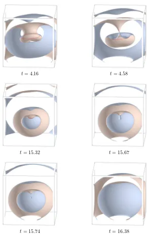
t= 15.74 t= 16.38
Figure 8: Scroll ring annihilation. By t = 4.2, a spiral-like cross-section has formed. The scroll ring emits ball shaped target waves twice per revolution, starting at approximatelyt= 4.58. After scroll ring annihilation att0= 23.45, the surfaceu
1 = 0 largely follows a concentric target wave pattern rather than a scroll ring pattern. The remaining target waves move outwards, and the medium becomes quiescent.
MPEG-Movie [10.7MB,gzipped]
t= 6.13 t= 17.875
t= 31.60 t= 35.654
t= 36.446 t= 39.918
Figure 9: Collision of scroll waves: Two scroll wave filaments drift towards each other. After t = 17, they start interacting visibly. Around t = 34, the filaments have found a common tangent plane and start lining up for collision. The crossover collision occurs at t0 = 35.83, x0 = (−3.25,3.25,0). After collision, the filaments connect adjacent faces of the cube rather than opposite faces.
MPEG-Movie [10.6MB,gzipped]
which has zeros in [−π/2, π/2]3 at (0, x
2,−π/6) and at (x1,0, π/6). Taking
u0=σ◦γ, we then start with explicit initial conditions
u1
0(x) = sin(ax1)(ax3−π/6) + sin(ax2)(ax3+π/6),
u2
0(x) = 0.25∗(sin(ax1) sin(ax2)−(ax3+π/6)(ax3−π/6)).
(8.18)
The spatial scaling factorais chosen asπ/20.
This example was selected because (8.17) has zeroes in [−π/2, π/2]3 at (0, x2,−π/6) and at (x1,0, π/6). Then (u01, u20) has zeroes at (0,x˜2,−10/3)
and at (˜x1,0,10/3). Therefore, att= 0, filaments are at right angles to each
other. Near resonant forcing with amplitudeA= 0.01 and frequencyω= 3.92 is chosen, together with an appropriate initial phase, such that the filaments drift towards each other and eventually interact.
Under discretization, crossover collision occurs at
t0= 35.83; x0= (−3.25,3.25,0).
(8.19)
For illustration/animation see figures 9 and 10.
Naively, there would be at least two options for non-destructive collision of the two scroll wave filaments. In figures 4, 9 and 10, the two primary filaments are seen to touch, forming a crossing with four emanating semi-branches. Keeping their orientation, the semi-branches could either simply re-connect, as before the collision. Alternatively, they could separate and connect with that semi-branch of matching orientation which they were not attached to previously. The first scenario of a crossing collision may be more intuitive at first: the two incoming semi-branches simply reconnect to their previous outgoing partners without exchangingtheir pairing. Such a crossing clearly would not change the global connectivity of the filaments. Viewed in projection onto the tangent planeEat collision timet0, however, the filament branches would then have to
remain crossing immediately before and after collision timet0, in contradiction
to both theorem 2.2 and numerical observation in figures 9 and 10.
Note that the filaments, albeit initially straight lines, have to bend out of their way considerably in order to accommodate a generic crossover collision in the tangent plane E. Indeed, initial conditions, periodic forcing, and boundary conditions are all chosen invariant under a rotation by 180o around the axis
Awhich diagonally connects the mid-edge points (−10,10,0) and (10,−10,0) of the domain Ω. This rotation invariance is preserved by the solution u(t, .). Because rotation initially maps one filament into the other, the collision point x0 must occur on the axis A – and it does, see (8.19). Similarly, the tangent
planeE must be orthogonal toA, forming angles of 45owith the straight line
initial conditions. We found it fascinating to watch the numerical filaments obey all these predictions.
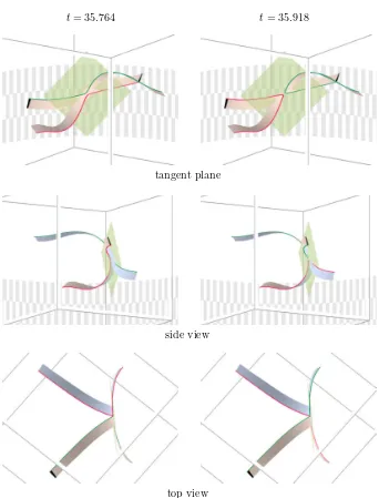
t= 35.764 t= 35.918
tangent plane
side view
top view
Figure 10: Details of the crossover collision: breaking and reconnecting scroll wave filaments, consistently with theorem 2.2. The two incoming semi-branches ex-changetheir pairing with the two outgoing semi-branches att =t0, x=x0. Each incoming semi-branch crosses over to its opposite outgoing semi-branch. The pro-jected branches, when viewed locally in the tangent planeE= kerux to the collision configuration att=t0, x=x0, neither cross before nor after collision.
MPEG-Movie [10.7MB,gzipped]
k-jets, again based on transversality, lemma 3.1. The present example and its codimension, however, comply with our simple rotation symmetry. In the coordinates (1.6) of crossover collision this can be seen from invariance under the 180orotation (x
1, x2)7→(−x1,−x2) around thex3 axis.
8.5 Collision of linked twisted scroll rings
In the previous non-autonomous example we have seen how crossover collisions change the local connectivity of tip filaments. We now present an autonomous example, with forcing amplitudeA= 0, where two linked filaments merge into a single filament. After collision the resulting filament is neither knotted nor self-linked but is isotopic to a circle.
We start with initial conditions u0 prescribed by (8.14), with the polynomial
p=z2
1−z22 and stereographic scaling factorc= 8/21 in (8.12).
p = z12−z22,
c = 8/21. (8.20)
Under discretization, crossover collision occurs at
t0= 4.90, x0= (0,0,−2.14)
(8.21)
For illustration/animation see fig. 11.
We comment on the changes of the global topological characteristics of twist and linking which occur at the crossover collision in this example. See figure 12 for a caricature of the essential features.
To determine the twist of a non self-intersecting closed oriented filament ϕt,
we first orient the tip filament ϕt as described in section 7. Then we count
the integer winding number of the accompanying isochrone bandχtaroundϕt,
according to the right hand rule. The integer twist can be positive, negative, or zero. Next suppose the filamentϕtspans an embedded disk, as all filaments in
figures 11, 12 do. The orientation ofϕtinduces an orientation of the disk which,
again by the right hand rule, we can represent by a field of vectorsν normal to the disk. To any other oriented filament crossing the disk transversely, we associate a crossing sign +1, if the crossing is in the direction of ν, and −1 otherwise. Following [40], the sum of crossing signs on the disk adds up to the twist of the boundary filamentϕt.
Applied to the schematic representation of figure 11 in figure 12, we conclude that the two filamentsϕt
ℓ, ϕtrfort < t0each have twist−1. After collision the
single remaining filament is untwisted. Our example therefore indicates that one can hope, at best, for a conservation of the parity of the total twist.
8.6 Unknotting the trefoil knot by crossover collision
t= 0.00 t= 1.665
t= 4.278 4.881
t= 4.910 t= 10.598
Figure 11: Crossover collision of two linked twisted filaments att0= 4.90, x0 = (0,0,−2.14) into a single untwisted filament.
MPEG-Movie [3.3MB,gzipped]
ϕt
ℓ ϕtr
Figure 12: A caricature of the crossover collision of two linked, simply twisted filamentsϕtℓ, ϕ
t
r att=t0. Before collision, each scroll ring possesses a twist of −1. After collision, the resulting scroll ring is untwisted, globally.
of the equations. In contrast, we now take a trefoil knot as an initial condition that already exhibits fully developed scroll waves. We then rescale space, which is equivalent to a change of diffusion constants. This brings the filaments into sufficiently close contact for interaction.
The initial conditions for this autonomous example,A= 0, are the numerical end state of a coarser simulation on a domain Ω1 = [−25,25]3, also running
on a numerical grid of 1253 grid points. The initial condition for the coarser
simulation (starting at timet=−10) is created using the polynomialp=z2 1−z23
with stereographic scaling factorc= 1/5 in (8.12):
z1 = 1/5(x1+ix2);
z2 = 1/5x3+i((x21+x22+x23)/52−1/4);
u1
0(x) = Re(z12−z23) clamped by (8.7);
u2
0(x) = 0.25Im(z12−z32) clamped by (8.7).
(8.22)
At timet= 0, we stop the simulation, keeping the same numerical data at grid points but rescaling the domain to Ω = [−15,15]3. This is the initial condition
at t= 0.
Under discretization, crossover collision from a trefoil knot to two linked rings is observed at
t0= 8.94, x0= (0,0,−9.28)
(8.23)
For illustration/animation see figure 13. Again we provide a caricature in figure 14.
8.7 Discussion of examples
We conclude our series of examples with some remarks. Concerning example 8.3 of scroll ring annihilation we observe that only untwisted scroll rings can be directly annihilated. This follows from the normal form of the corresponding singularity with positive definite quadratic formhP ut, P uxx|Eiat (t0, x0); see
t= 0.00 t= 4.905
t= 7.985 t= 8.914
t= 8.966 t= 12.597
Figure 13: Decomposing the trefoil knot into two linked twisted unknotted fila-ments by crossover collision att0= 8.94, x0= (0,0,−9.28). As explained in example 8.3, we see in figures 13, 14 how the trefoil knot with twist±3 decomposes into two unknotted, but mutually linked twisted filaments, each of twist −1.
MPEG-Movie [8.9MB,gzipped]
Figure 14: A caricature of the unknotting of the trefoil knot, showing the orien-tations of all filaments.
require a three-dimensional kernel and hence a singularity of codimension at least six.
We have not presented an example for the process opposing annihilation: the creation of a circular filament by a negative definite quadratic form hP ut, P uxx|Eiat (t0, x0). Since the definiteness required for P uxx|E does not
predetermine the direction of △u, we could construct initial conditions u0(x)
corresponding to scroll ring creation at t0 = 0, x0 ∈ Ω. Although we expect
scroll ring creation to be feasible also for large positive times t0, we did not
observe this phenomenon in our simulations so far.
Our results provide specific examples of the “internal” collision type, which [31] have described as topologically viable; furthermore, we show that crossover collision is the only generic way for scroll waves to change their topological linking type.
From a modeling point of view, experimental systems may require substantially more than just two dependent variables u1, u2 for an adequate description by
parabolic reaction diffusion systems. We repeat that theorem 4.2 predicts the described two-variable phenomena to occur in any projection setting, where only two combinations of the relevant quantitiesu1, ..., um are observable, for
example by color shading. We emphasize that this observation neither requires, nor corresponds to, a dynamic reduction of the full underlying reaction diffusion system by inertial manifolds or related techniques of dimension reduction. Aiming at the ubiquitous wealth of phenomena of pattern formation and pat-tern transformation, our paper has detected and addressed just a few elemen-tary dynamic effects peculiar to systems of two equations in three space di-mensions. Clearly, the theoretical framework supports significantly more com-plicated spatio-temporal effects than were presented here. Applicability hope-fully also will reach far beyond the specific motivating context of Belousov-Zhabotinsky patterns or excitable media.
References
[1] R. Abraham and J. Robbin. Transversal Mappings and Flows. Benjamin, New York, 1967.
[3] S. Angenent. The zero set of a solution of a parabolic equation Crelle J. reine angew. Math., 390:79–96, 1988.
[4] D. Barkley. Spiral meandering. In Chemical Waves and Patterns, R. Kapral and K. Showalter (eds.), 163–190. Kluwer, 1995.
[5] D. Barkley, M. Kness, and L. S. Tuckerman. Spiral-wave dynamics in a simple model of excitable media - the transition from simple to compound rotation. Phys. Rev. A, 42:2489–2492, 1990.
[6] K. Brauner. Zur Geometrie der Funktionen zweier komplexer Ver¨ ander-licher iii,iv. Abh. Math. Sem. Hamburg, 6:8–54, 1928.
[7] J. Damon. Local Morse theory for solutions to the heat equation and Gaussian blurring. J. Diff. Eqns., 115:368–401, 1995.
[8] J. Damon. Generic properties of solutions to partial differential equations. Arch. Rat. Mech. Analysis, 140:353–403, 1997.
[9] J. Damon. Singularities with scale threshold and discrete functions ex-hibiting generic properties. Mat. Contemp., 12:45–65, 1997.
[10] J. Dieudonn´e. Elements d’Analyse 2. Gauthier-Villars, Paris, 1969.
[11] M. Dowle, R. M. Mantel, and D. Barkley. Fast simulations of waves in three-dimensional excitable media. Int. J. Bifur. Chaos, 7:2529–2546, 1997.
[12] B. Fiedler and C. Rocha. Orbit equivalence of global attractors of semilin-ear parabolic differential equations.Trans. Amer. Math. Soc., 352:257-284, 2000.
[13] B. Fiedler and D. Turaev. Normal forms, resonances. and meandering tip motions near relative equilibria of Euclidean group actions. Arch. Rat. Mech. Analysis, 145:129–159, 1998.
[14] A. Friedman. Partial Differential Equations. Holt, Reinhart & Winston, New York, 1969.
[15] M. Golubitsky and D. G. Schaeffer. Singularities and Groups in Bifurca-tion Theory I. Appl. Math. Sc. 51, Springer-Verlag, 1985.
[16] D. Henry. Geometric Theory of Semilinear Parabolic Equations. Springer-Verlag, Berlin, 1981.
[17] C. Henze and J. J. Tyson. Cellular-automaton model of 3-dimensional excitable media. J. Chem. Soc. Farad. Transac., 92:2883–2895, 1996.
[18] C. Henze and A.T. Winfree. A stable knotted singularity in an excitable medium. Int. J. Bif. Chaos, 1:891–922, 1991.
[19] M. W. Hirsch. Differential Topology. Springer-Verlag, New York, 1976.
[21] O. A. Ladyzhenskaja, V. A. Solonnikov, and N. N. Ural´ceva. Linear and Quasilinear Equations of Parabolic Type. Moscow, 1967. English: AMS, Providence, 1968.
[22] R. M. Mantel and D. Barkley. Periodic forcing of scroll-wave patterns in three-dimensional exciatable media. Preprint, University of Minnesota, IMA #1568, 1998.
[23] H. Matano. Nonincrease of the lap-number of a solution for a one-dimensional semi-linear parabolic equation. J. Fac. Sci. Univ. Tokyo Sec. IA, 29:401–441, 1982.
[24] A. V. Panfilov, A. N. Rudenko, and V. I. Krinsky. Turbulent rings in 3-dimensional active media with diffusion by 2 components. Biofizika, 31:850–854, 1986.
[25] A. V. Panfilov and A. T. Winfree. Dynamical simulations of twisted scroll rings in 3-dimensional excitable media. Physica D, 17:323–330, 1985. [26] A. Pazy.Semigroups of Linear Operators and Applications to Partial
Dif-ferential Equations. Springer-Verlag, New York, 1983.
[27] D.G. Schaeffer. A regularity theorem for conservation laws. Adv. Math., 11:368–386, 1973.
[28] C. Sturm. Sur une classe d’equations a difference partielles. J. Math. Pure Appl., 1:373–444, 1836.
[29] H. Tanabe. Equations of Evolution. Pitman, London, 1979.
[30] R. Thom. Un lemma sur les applications differentiables. Bol. Soc. Mat. Mex., 2:59–71, 1956.
[31] J. J. Tyson and S. H. Strogatz. The differential geometry of scroll waves. Int. J. Bif. Chaos, 1:723–744, 1991.
[32] J. R. Weimar, J. J. Tyson, and L. T. Watson. 3rd generation cellular automaton for modeling excitable media. Physica D, 55:328–339, 1992. [33] J. R. Weimar, J. J. Tyson, and L. T. Watson. Diffusion and
wave-propagation in cellular automaton models of excitable media. Physica D, 55:309–327, 1992.
[34] N. Wiener, A. Rosenblueth. The mathematical formulation of the problem of conduction of impulses in a network of connected excitable elements, specifically in cardiac muscle. Arch. Inst. Cardiol. Mexico, 16:205-265, 1946.
[35] A. T. Winfree. Spiral waves of chemical activity. Science, 175:634–636, 1972.
[36] A. T. Winfree. Scroll-shaped waves of chemical activity in three dimen-sions. Science, 181:937–939, 1973.
[38] A. T. Winfree. Varieties of spiral wave behavior: An experimentalist’s approach to the theory of excitable media. Chaos, 1:303–334, 1991. [39] A. T. Winfree. Persistent tangles of vortex rings in excitable media.
Phys-ica D, 84:126–147, 1995.
[40] A. T. Winfree, E. M. Winfree, and M. Seifert. Organizing centers in a cellular excitable medium. Physica D, 17:109–115, 1985.
Bernold Fiedler
Institut f¨ur Mathematik I Freie Universit¨at Berlin Arnimallee 2-6
D-14195 Berlin, Germany [email protected]
Rolf M. Mantel
Philipps-Universit¨at Marburg
Fachbereich Mathematik und Informatik Hans-Meerwein Str.
35032 Marburg

![Figure 7:Interaction and collision of a pair of spiral waves in the plane.MPEG-Movie [26.4MB,gzipped]](https://thumb-ap.123doks.com/thumbv2/123dok/923627.902785/24.595.130.471.178.595/figure-interaction-collision-spiral-waves-plane-movie-gzipped.webp)

![Figure 11:Crossover collision of two linked twisted filaments at t0 = 4.90, x0 =(0, 0, −2.14) into a single untwisted filament.MPEG-Movie [3.3MB,gzipped]](https://thumb-ap.123doks.com/thumbv2/123dok/923627.902785/31.595.129.470.185.603/figure-crossover-collision-twisted-laments-untwisted-lament-gzipped.webp)
