Full Terms & Conditions of access and use can be found at
http://www.tandfonline.com/action/journalInformation?journalCode=ubes20
Download by: [Universitas Maritim Raja Ali Haji] Date: 11 January 2016, At: 18:53
Journal of Business & Economic Statistics
ISSN: 0735-0015 (Print) 1537-2707 (Online) Journal homepage: http://www.tandfonline.com/loi/ubes20
Bayesian Inference in Regime-Switching ARMA
Models With Absorbing States: The Dynamics of
the Ex-Ante Real Interest Rate Under Regime Shifts
Chang-Jin Kim & Jaeho Kim
To cite this article: Chang-Jin Kim & Jaeho Kim (2015) Bayesian Inference in Regime-Switching ARMA Models With Absorbing States: The Dynamics of the Ex-Ante Real Interest Rate Under Regime Shifts, Journal of Business & Economic Statistics, 33:4, 566-578, DOI: 10.1080/07350015.2014.979995
To link to this article: http://dx.doi.org/10.1080/07350015.2014.979995
Accepted author version posted online: 06 Nov 2014.
Published online: 27 Oct 2015. Submit your article to this journal
Article views: 134
View related articles
Bayesian Inference in Regime-Switching ARMA
Models With Absorbing States: The Dynamics
of the Ex-Ante Real Interest Rate Under
Regime Shifts
Chang-Jin K
IMDepartment of Economics, University of Washington, Seattle, WA 91895 ([email protected])
Jaeho K
IMDepartment of Economics, University of Oklahoma, Norman, OK 73019 ([email protected])
One goal of this article is to develop an efficient Metropolis–Hastings (MH) algorithm for estimating an ARMA model with a regime-switching mean, by designing a new efficient proposal distribution for the regime-indicator variable. Unlike the existing algorithm, our algorithm can achieve reasonably fast convergence to the posterior distribution even when the latent regime-indicator variable is highly persistent or when there exist absorbing states. Another goal is to appropriately investigate the dynamics of the latent ex-ante real interest rate (EARR) in the presence of structural breaks, by employing the econometric tool developed. We show that excluding the theory-implied moving-average terms may understate the persistence of the observed EPRR dynamics. Our empirical results suggest that, even though we rule out the possibility of a unit root in the EARR, it may be more persistent and volatile than has been documented in some of the literature.
KEY WORDS: Global Metropolis-Hastings algorithm; Proposal distribution.
1. INTRODUCTION
The ex-ante real interest rate (EARR) is a key economic variable, which affects economic agents’ intertemporal con-sumption, savings, and investment decisions. Its dynamics play a central role in many theoretical models such as asset pric-ing models, and macro dynamic stochastic general equilibrium (DSGE) models. Thus, understanding the behavior of the EARR has been a crucial issue in the literature, as surveyed in Neely and Rapach (2008).
The seminal article by Fama (1975) provides striking empir-ical evidence that U.S. EARR is essentially constant. Nelson and Schwert (1977) and Garbade and Wachtel (1978), however, challenged Fama’s (1975) finding by showing that his statisti-cal test is not informative enough to conclude the behavior of the EARR and raised the possibility of a time-varying EARR. Subsequent studies by Mishkin (1981), Huizinga and Mishkin (1986), and Antoncic (1986), also showed that the empirical result of constant U.S. EARR is critically dependent upon a particular sample period and thus, it is hard to confirm Fama’s (1975) argument. Building upon those empirical findings, Rose (1988) even raised the possibility that the EARR may be an I(1) process. Since Rose (1988) raised the issue, the literature has reported mixed results. By applying various unit root and cointegration tests to the ex-post real interest rate (EPRR), King et al. (1991), Gali (1992), Mishkin (1992), and Koustas and Ser-letis (1999) concluded that the EARR is nonstationary with a unit root. (Under rational expectations, a unit root in the EARR implies a unit root in the EPRR.) On the other hand, Crowder and Hoffman (1996), and Rapach and Weber (2004) argued that the EARR is stationary but highly persistent. Additionally, Sun
and Phillips (2004) showed that the EARR has mean-reverting dynamics with long-memory properties, based on fractional integration tests.
Another strand of the empirical literature on this issue is to investigate the implications of regime shifts in the real interest rates on the persistence of the EARR. Note that Perron (1990) argued that a failure to account for mean shifts may lead to spurious evidence of high persistence for a series under consid-eration. Thus, Caporale and Grier (2000) and Bai and Perron (2003) confirmed that the unit root hypothesis can be rejected if shifts in the mean are allowed for the EPRR, suggesting that the EARR is stationary. By incorporating regime shifts or structural breaks in the mean of the EARR in an autoregressive model of the EPRR, Garcia and Perron (1996) even showed that the EARR may be a constant subject to occasional jumps caused by important structural events.
One goal of this article is to appropriately investigate the dy-namics of the EARR, in the presence of structural breaks in its mean with unknown break points. Under the maintained hy-pothesis of rational expectations, if we assume that the EARR follows an AR(2) process then the EPRR follows an autoregres-sive moving average (ARMA) (2,2) process. This is because the EPRR is a sum of an AR(2) process for the EARR and a seri-ally uncorrelated inflation forecast error. We argue that omitting the moving average terms as in Garcia and Perron (1996) may
© 2015American Statistical Association Journal of Business & Economic Statistics
October 2015, Vol. 33, No. 4 DOI:10.1080/07350015.2014.979995
Color versions of one or more of the figures in the article can be found online atwww.tandfonline.com/r/jbes.
566
result in misleading inference about the dynamics of the EARR. Furthermore, approximating the moving-average components in the EPRR with a finite-order autoregressive process would result in size distortions in testing for a unit root. If the EPRR follows an ARMA(2,2) process with a regime-switching mean, however, estimation of the model is not as straightforward as in Garcia and Perron’s (1996) regime-switching model, in which the moving average terms implied by the rational expectations theory are omitted.
Another goal of this article is to develop an efficient Bayesian method for estimating an ARMA model with a regime-switching parameters, which will be used as an econometric tool to be employed in achieving the goal of investigating the dynamics of the EARR. In case the disturbance terms are iid within a regime, the approximate maximum likelihood estimation of the model is readily available based on the state-space representa-tion of the model, as proposed by Kim (1994). However, with heteroscedastic disturbances within a regime, estimation of the model is infeasible within the classical framework, leading us to resort to the Bayesian approach.
Our Bayesian approach builds on the work of Billio, Mon-fort, and Robert (1999) in that we effectively incorporate their global Metropolis-Hastings (MH) algorithm. That is, at each iteration of the Markov chain Monte Carlo (MCMC) algorithm, the whole sequence of the state or the latent regime-indicator variable is drawn from the proposal distribution, which can rea-sonably approximate the target distribution, conditional on all the parameters of the model and data. (Throughout the arti-cle, we focus on generating the regime-indicator variablesSt,
t=0,1,2, . . . , T, conditional on the parameters of the model. We resort to Chib and Greenberg (1994) and Nakatsuma (2000), for making inferences about the parameters of the model con-ditional on the regime-indicator variables and data.) Then, the approximation error in the proposal distribution is corrected for by globally accepting or rejecting the newly drawn regime-indicator variables according to an appropriately defined ac-ceptance probability. Both Billio, Monfort, and Robert (1999) algorithm and ours are multi-move samplers in the sense that the transition of the MH Markov chain involves all the state variable in one block. However, our algorithm is different from theirs in that we employ a more efficient proposal distribu-tion. (Recently, other researchers have also proposed efficient multi-move sampling methods for Markov switching dynamic models. Refer to Fruehwirth-Schnatter (2006) for issues related to mixture and Markov-switching models; Fiorentini, Planas, and Rossi (2012) for multi-move sampling in dynamic mix-ture models; Bauwens, Dufays, and Rombouts (2014) for par-ticle MCMC; and Billio, Casarin, and Osuntuy (in press) for multiple-try Metropolis-sampling for Markov switching gener-alized autoregressive conditional heteroscedasticity (GARCH) models.)
One potential source of inefficiency of Billio, Monfort, and Robert (1999) global MH algorithm is that their joint state pro-posal distribution is the product of individual propro-posal distribu-tions of the hidden state, and that each individual state distri-bution depends on the neighboring states and accounts for the information from the data only through the current observation. Another source of inefficiency is due to the global accept/reject
step that could lead to very low acceptance rates when the pro-posal distribution is not very well designed. In this article, we solve the problem of inefficiency by designing a new efficient proposal distribution. In addition, the low acceptance rate of the global MH algorithm is solved as a consequence of the choice of a new proposal distribution. (We appreciate the anonymous referees for mentioning these points clearly.) We note that, when sampling the states or the regime-indicator variables from the proposal distribution, Billio, Monfort, and Robert (1999) em-ployed a single-move sampler and we employ a multi-move sampler.
As theoretically proven by Liu, Wong, and Kong (1994) and Scott (2002), a multi-move sampler significantly reduces the au-tocorrelations among successive draws of the regime-indicator variables and other parameters of the model in MCMC itera-tions. Carter and Kohn (1994), Shephard (1994), and De Jong and Shephard (1995) empirically showed that the multi-move samplers are more efficient than the single-move samplers, in the sense that convergence to the posterior distribution will be faster. Even though both Billio, Monfort, and Robert (1999) algorithm and ours are fundamentally multi-move samplers, the choice of the proposal density can affect the convergence of the samplers considerably. Actually, there is a case in which the algorithm based on Billio, Monfort, and Robert (1999) proposal distribu-tion results in no convergence to the posterior distribudistribu-tion at all in a regime-switching ARMA model. This is the case when there exist absorbing states. With absorbing states, correlations between two subsequent latent regime-indicator variables are perfect or almost perfect. As a result, the desired asymptotic posterior distribution is never achieved if the states are gener-ated from the proposal distribution via the single-move sampler. Garcia and Perron (1996), in their maximum likelihood estima-tion of a three-state Markov-switching AR model for the EPRR, showed that their estimates of the transition probabilities imply existence of structural breaks with two absorbing states. Thus, with absorbing states or structural breaks in the mean of our ARMA process for the EPRR, the single-move sampler would never achieve convergence. We show that our MH algorithm can achieve reasonably fast convergence even in such a case, as we employ the multi-move sampler when sampling the states from the proposal distribution.
The remainder of the article is organized as follows. Section2 presents our benchmark econometric model and provides a liter-ature review on the inference of regime-switching ARMA mod-els. Section3provides a new efficient MCMC algorithm based on a multi-move sampler, for drawing the Markov-switching regime-indicator variables conditional on all parameters of the model. In Section 4, we perform simulation studies to eval-uate the performance of the proposed Bayesian algorithm. In particular, we show that our sampler achieves reasonably fast convergence, even in the case in which Billio, Monfort, and Robert (1999) sampler fails to converge at all. In Section 5, the benchmark model in Section 2 is extended to incorporate stochastic volatility in the disturbance terms, and then the ex-tended model is applied to investigate the dynamics of the la-tent EARR by estimating a regime-switching ARMA model for the EPRR. Section5 provides a summary and concluding remarks.
2. MODEL SPECIFICATION AND LITERATURE REVIEW ON MARKOV-SWITCHING ARMA MODELS:
CRITIQUE
Consider the following ARMA(p, q) model with dependent coefficients (We focus on generating the regime-indicator variables St, t=0,1,2, . . . , T, conditional on the
parameters of the model and data. We present the MCMC algo-rithm for generating the parameters of the model conditional on the regime-indicator variables and data inAppendix A, by com-plementing those in Chib and Greenberg (1994) and Nakatsuma (2000).):
where the subscriptSt suggests that the corresponding
coeffi-cient is dependent on a latent regime-indicator variableSt. We
assume thatStfollows anM-state first-order Markov switching
process with the following transition probabilities:
Pr[St =j|St−1 =i]=pij, Note that, by restricting the transition probabilities of the above regime-switching model appropriately to allow for ab-sorbing states, one can design a model of structural breaks with unknown break points, as suggested by Chib (1998). Later in Section5, an extended version of this model is applied to the EPRR. To deal with the non-iid nature of the shocks to the EPRR within a regime, the model will be extended to allow for stochastic volatility in the disturbance terms. For simplicity of exposition, we stick to the above model specification in this section.
Due to its non-Markovian nature, the above model is not easy to estimate. Within the classical framework, for example, evaluation of the likelihood function is not feasible without resorting to some sort of approximation. This is because the conditional density of yt depends upon the entire history of
the latent regime-indicator variable up to time t. To get over this problem, we can first cast the above model into a state-space model. We can then employ the approximate Kalman filter algorithm proposed by Kim (1994). The basic idea in Kim (1994) is to employ an approximation to the conditional density ofyt, so that it can be dependent only onSt =j and
St−1=i, (i, j=1,2, . . . , M) at each iteration of the Kalman filter. His method is easy to implement for the above model with iid disturbance terms. However, if the above model is extended to deal with stochastic volatility in the disturbance terms, his approach is no longer applicable. Only within the Bayesian framework, is estimation of the extended model feasible.
Within the Bayesian framework, Billio, Monfort, and Robert (1999) proposed an MCMC algorithm for sampling the regime-indicator variablesSt,t =0,1,2, . . . , T, from a proposal
dis-tribution, which can approximate the target distribution. Then, they correct for the approximation error in the proposal distri-bution by employing the MH algorithm. (Readers are referred
to Chib and Greenberg (1995), Gilks, Richardson, and Spiegel-halter (1996), and Koop (2003) for the MH algorithm and ref-erences therein.) For example, once the whole sequence of the regime-indicator variable is drawn from the proposal distribu-tion, the approximation error is corrected for by globally ac-cepting or rejecting the newly drawn regime-indicator variables according to an appropriately defined acceptance probability. In drawing the regime-indicator variables from the proposal distribution, Billio, Monfort, and Robert (1999) resorted to a single-move sampler, in which a single indicator variableSt is
drawn one at a time fort =0,1,2, . . . , T, conditional on the remaining regime-indicator variablesS1,S2,...,St−1,St+1,...,ST.
In what follows, we provide a review of Billio, Monfort, and Robert (1999) algorithm.
Review of the MCMC Algorithm by Billio, Monfort, and
Robert (1999)
For a direct single-move Gibbs sampler, one can theoretically drawSt, fort =0,1,2, . . . , T, from probabilities. The validity of going from the second line to the third line is ensured by the Markov property ofSt. As we go
from the third line to the fourth line, all irrelevant future states, Sτ,τ =t+1, . . . , T, are dropped. For an AR(p) process
with-out a moving-average term in Albert and Chib (1993), Equation (4) can be simplified as
However, for each generation of St one needs to
evalu-ate the individual likelihood functions f(yk|S˜k,Y˜k−1), k= t, t+1, . . . , T. This means that the sampling scheme requires O(T(T2+1)) operations. Consequently, as the number of regimes
or the sample size increases, the algorithm becomes infeasible as computational costs increase exponentially.
To get over the problem, Billio, Monfort, and Robert (1999) proposed an MH algorithm as an alternative to the direct Gibbs sampling approach. Instead of generating individualSt directly
from the distribution in Equation (4) fort =0,1,2, . . . , T, they proposed to generate it from the following individual proposal distribution: which is an approximation to the individual target distribution in Equation (4). As the above distribution depends only on the density of yt, generating ˜St is an O(T) algorithm unlike the
Gibbs sampling approach based on Equation (4).
As the above individual proposal densities are based on ap-proximations, Billio, Monfort, and Robert (1999) proposed to employ the MH algorithm. Once a candidate ˜S is drawn from the individual candidate densities, the approximation errors can be corrected for by globally accepting or rejecting the generated
˜
STaccording to an appropriately defined acceptance probability.
By defining ˜SJ
T to be the newly generated set of ˜ST and ˜STJ−1to
be an accepted set of ˜STat the previous iteration of the sampler,
the acceptance probability is defined as
α˜ where, by considering the normalizing constants, the proposal distributionG( ˜ST|Y˜T) is given by terms, Billio, Monfort, and Robert (1999) derived the following acceptance probability: Note again that Billio, Monfort, and Robert (1999) employed a single-move sampler when sampling the state variables from the proposal distribution. As discussed in Liu, Wong, and Kong (1994) and Scott (2002), however, a potential weakness of the single-move sampler is that its performance gets worse with slower mixing as the persistence of the latent state variable in-creases. (In probability theory, the mixing time of a Markov chain means the time until the Markov chain reaches the steady-state distribution. The mixing time determines the running time for simulation.) Furthermore, slower mixing for the regime-indicator variables translates into slower mixing for the param-eters of the model as well, according to a duality principle
introduced by Diebolt and Robert (1994). Actually, our simula-tion study in Secsimula-tion4shows that there are cases in which the single-move sampler results in no convergence to the posterior distribution at all. This happens when the Markov-switching regime-indicator variable is highly persistent or when there ex-ists an absorbing state, as in Garcia and Perron (1996).
3. AN EFFICIENT MCMC ALGORITHM BASED ON A
NEW PROPOSAL DISTRIBUTION
In this section, we attempt to get over the weaknesses of Billio, Monfort, and Robert (1999) algorithm by implementing a multi-move sampler when sampling the state variables from the proposal distribution. Note that a successful implementation of the MH algorithm depends critically upon the appropriate derivation of a proposal distribution that reasonably approxi-mates the target distribution. We thus consider the following decomposition of the target distributionF( ˜ST|Y˜T):
Theoretically, the above decomposition suggests that one can sequentially generateST fromf(ST|Y˜T), and thenSt from the
conditional distributionf(St|S˜t+1:T,Y˜T), fort =T −1, . . . ,0.
By defining ˜Yt =[y1y2. . . yt]′and ˜Yt+1:T =[yt+1yt+2. . . yT]′,
this conditional distribution can be derived as f
However, evaluating the above distribution is not feasible in the presence of a nontrivial moving-average structure. Thus, we propose to sequentially generateSt,t =T , T −1, . . . ,1,0,
from the individual proposal distribution given below, as an approximation to the density in Equation (12):
g
below. An additional approximation involved is that we ignore T
k=t+1f(yk|S˜t:k,Y˜k−1) from Equation (12).
Building upon ideas in Hamilton (1988,1989), Cosslett and Lee (1985), and Harrison and Stevens (1976), Kim (1994) pre-sented filtering and smoothing algorithms for a state-space model with Markov switching, along with maximum likeli-hood estimation of the unknown parameters of the model. In particular, by combining the Hamilton filter (1989) and an
approximate Kalman filter, he provided an algorithm for ob-taining h(St|Y˜t) as an approximation to f(St|Y˜t) for a
gen-eral state-space model with Markov switching. Note that an ARMA model with Markov switching can always be cast into a state-space model with Markov switching. For details of Kim’s (1994) approximate Kalman filter and algorithm for calculating h(St|Y˜t) as an approximation tof(St|Y˜t), readers are referred to
Appendix B.
Once ˜ST is generated from the proposal distribution in
Equa-tion (13), we follow Billio, Monfort, and Robert (1999) in adopt-ing a global MH approach to correct for the approximations involved in our proposal distribution. We accept or reject glob-ally the whole sequence ofS0, S1, . . . , ST, using an appropriate
acceptance probability. Let ˜SJ T and ˜S
J−1
T be the sequences of
S0, S1, . . . , ST generated at the current and the previous
itera-tions of the MCMC algorithm, respectively. Then, the accep-tance probability is given by
α˜ and G(.|Y˜T) is the multi-move proposal distribution defined
below: we can derive the following acceptance probability:
α˜
filter of Kim (1994) to the state-space model representation of the Markov-switching ARMA model; and f(yt|S˜t,Y˜t−1) can be evaluated by applying the conventional Kalman filter to the state-space model. What follows describes a brief summary of the MH algorithm for generating ˜ST.
Summary of Metropolis-Hastings Algorithm for Generating
˜
ST at the Jth Iteration
(i) We cast the Markov-switching ARMA model into a space form, conditional on all the parameters. For a
state-space representation of the model, readers are referred to Appendix B.
(ii) We apply the approximate filter in Kim (1994) to the state-space representation of the model to evaluate and save h(St|Y˜t) andh(St+1|Y˜t). In this step, we also calculate and
save h(SJ−1
t |Y˜t) and h(StJ+−11|Y˜t), whereStJ−1 andS J−1
t+1 refer to the regime-indicator variables generated at the previous iteration of the sampler.
(iii) Using h(St|Y˜t) andh(St+1|Y˜t) saved from (ii), we
gen-erate St sequentially in the backward direction fort =
T , T −1, . . . ,1,0, based on the individual proposal
dis-(iv) We apply the conventional Kalman filter again to the state-space model representation of the model condi-tional on ˜ST =S˜TJ, to evaluate and savef(yt|S˜tJ,Y˜t−1), t =1,2, . . . , T.
(v) We apply the conventional Kalman filter to the state-space model representation of the model conditional on ˜ST =
˜
STJ−1, to evaluate and savef(yt|S˜tJ−1,Y˜t−1).
(vi) Using the output from (ii) to (v), we calculate the accep-tance probability as in Equation (17). Then, we accept or reject ˜STJ according to this acceptance probability.
4. PERFORMANCE OF THE PROPOSED
ALGORITHM: SIMULATION STUDY
In this section, we compare the performances of the proposed algorithm and the Billio, Monfort, and Robert (1999) algorithm. For this purpose, we consider the following ARMA(1,1) model with a Markov-switching mean as a data-generating process:
yt =µSt +φ(yt−1−µSt−1)+et−θ et−1,
We fix all the parameters of the model except forp22 at the values given above. We then consider three cases that differ in the value of p22: for Case 1, we assignp22 =0.96; for Case 2, we assignp22=0.99; and for Case 3, we assign p22=1. For each of these three cases, we generate 50 datasets with the sample size of 300. (When generating data, elements of ˜ST
are assigned according to the expected duration of each regime calculated based on the assigned transition probabilities.) For each dataset generated, we apply both the proposed algorithm and the Billio, Monfort, and Robert (1999) algorithm.
For comparing the convergence of the two algorithms, we calculate Geweke’s (1992)z-score statistic for the posterior dis-tributions of thep11parameter. (We note that the results for the other parameters are very similar.) This test is designed to detect a convergence failure by comparing MCMC draws in the early part and the latter part of a Markov chain. The difference be-tween the posterior means is calculated from these two MCMC
subsamples and divided by its estimated standard error to ob-tain the statistic. For each algorithm, we obob-tain 120,000 MCMC draws after 5000 burn-ins. Then, these draws are equally di-vided into six subsamples. We denote ¯pτ11as the sample mean of theτth subsample ands(0)τas the asymptotic variance of the
sample mean as measured by the spectral density at frequency zero. Geweke’s (1992)z-score statistic is defined as
Zτ =
¯ p6
11−p¯
τ
11
s(0)6
n + s(0)τ
n
, τ =1,2, . . . ,5,
wheren=20,000.
Geweke (1992) showed that the test statistic asymptotically follows a standard normal distribution under the null hypothesis that convergence is achieved. For example, if the null hypothesis is not rejected forτ =1, we can conclude that convergence is achieved after 5000 iterations. If the null hypothesis is rejected forτ =5, it is an evidence that convergence will not be achieved even after 85,000 iterations.
The results are reported inTable 1. For the proposed algo-rithm, convergence is achieved within 45,000 iterations for the 96% of the datasets for all the three cases. However, for the Billio, Monfort, and Robert (1999) algorithm, convergence is not achieved even after 85,000 iterations for the 34% (74%) of the datasets for Case 1 (Case 2).
For Case 3, convergence is never achieved for any of the dataset. This is because we have an absorbing state for Case 3, and correlations between two subsequent states within regime 2 are perfect. As a result, the desired asymptotic posterior distri-butions are never achieved.
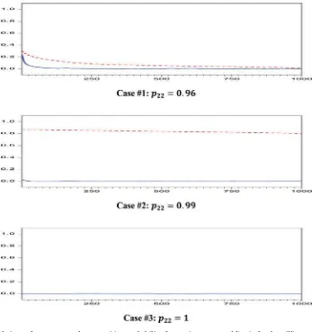
InFigure 1, the autocorrelations of the MCMC samples for p11are depicted for both algorithms. (Figure 1is prepared based on MCMC outputs for a particular sample for each case.) For Case 1, in which the state variableSt is not very persistent, the
autocorrelations die out fast for both algorithms. For Case 2, in which we have a more persistent state variable, the autocorrela-tions for our algorithm die out very quickly, while they die out very slowly with the Billio, Monfort, and Robert (1999)
algo-rithm. Note that, with our algorithm, the autocorrelations dies out very quickly even for Case 3.
5. UNCOVERING THE DYNAMICS OF U.S. EX-ANTE
REAL INTEREST RATE UNDER REGIME SHIFTS: 1960Q1–2008Q2
5.1 Model Specification for Ex-Post Real Interest Rate
Consider the following expression for the nominal interest rate (it):
it =rtEA+E[πt|It−1], (18) wherertEAdenotes the EARR;πtdenotes the inflation rate; and
E[πt|It−1] refers to economic agents’ rational expectation ofπt
conditional on all the available information up to periodt−1. Then the EPRR (rEP
t ) is given by
rtEP=rtEA−εt, (19)
whereεt=πt−E[πt|It−1] is inflation forecast error, which is serially uncorrelated under the rational expectations assumption.
We assume thatrEA
t follows an AR(2) process with a
regime-shifting mean, as given below: φ(L)
rtEA−µSt
=νt, (20)
whereφ(L)=(1−φ1L−φ2L2); the roots ofφ(L)=0 lie out-side the complex unit circle; νt is serially uncorrelated with
E(νt)=0; the subscript St refers to a latent regime-indicator
variable. Then, by subtractingµSt from both sides of Equation (19) and multiplying both sides of the resulting equation by φ(L), it is straightforward to show that the resulting EPRR fol-lows an ARMA(2,2) process with a Markov-switching mean, as given below:
rtEP=µSt +φ1
rtEP−1−µSt−1
+φ2
rtEP−2−µSt−2
+et−θ1et−1−θ2et−2, (21) where the roots of (1−θ1L−θ2L2)=0 lie outside the com-plex unit circle. Following Garcia and Perron (1996), we
fur-Table 1. Convergence diagnostics check [Geweke’s (1992)z-score test]
yt =µSt+φ(yt−1−µSt−1)+et−θ et−1, et∼iidN(0, σ2),
Pr[St=j|St−1=i]=pij, i, j=1,2,
p11=0.98; µ1=0.6; µ2=0; φ=0.3; θ=0.6; σ =0.2, t=1,2, . . . ,300.
Pr[|Zn| ≤1.96]
Case 1 (p22=0.96) Case 2 (p22=0.99) Case 3 (p22=1)
Burn-in Proposed Billio et al. Proposed Billio et al. Proposed iterations algorithm (1999) algorithm (1999) algorithm
5000 0.88 0.00 0.96 0.00 0.98
25,000 0.94 0.08 1 0.02 1
45,000 0.98 0.42 1 0.10 1
65,000 1 0.60 1 0.20 1
85,000 1 0.66 1 0.26 1
NOTES: 1. The number of MCMC draws is 20,000. 2. The reported results are based on 50 simulations.
3. Bayesian convergence diagnostic check is sequentially performed by increasing the number of burn-in iterations. The statistic is calculated based on MCMC draws ofp11.
Figure 1. Autocorrelations of MCMC samples: Transition probability for Regime 1. Dotted line is for the Billio et al. (1999) algorithm and solid line is for the proposed algorithm.
ther assume that the latent regime-indicator variable St
fol-lows a three-state, first-order Markov-switching process with the following transition probabilities:
Pr[St =j|St−1=i]=pij,
3
j=1
pij =1; i, j=1,2,3. (22)
To complete the model by accommodating the heteroscedas-tic nature of the shocks to the EPRR, we assume the following stochastic volatility for et (While Garcia and Perron (1996)
assumed a Markov-switching variance for et, we employ a
random-walk stochastic volatility, which is much more flexi-ble than a Markov-switching variance. To estimate the stochas-tic volatility, we implement the procedure proposed by Kim, Shepard, and Chib (1998) in our MCMC algorithm.):
et ∼N0, σt2
, (23)
lnσt2=lnσt2−1+ωt, ωt∼N
0, σω2, (24) whereωt is independent ofet.
Given the above model, we construct the EARR series by taking a conditional expectation of the EPRR:
E rtEPIt−1
=E µSt
It−1
+E ut
It−1
, (25)
where ut=φ1ut−1+φ2ut−2+et−θ1et−1−θ2et−2 and It−1 refers to information up to time t−1, which consists of all the current and past history of EPRR in the sample.
In this section, we employ the Bayesian econometric tool developed in Section 3, in estimating the above model for the U.S. EPRR. We use quarterly data on ex-post real inter-est, which is constructed by subtracting the consumer price index (CPI) inflation rate from the three-month Treasury bill rate. We extend Garcia and Perron’s (1996) sample to cover recent observations right before the financial crisis, and thus our sample covers the period of 1960Q1-2008Q2. All the inferences are based on 25,000 MCMC outputs, after 5000 burn-ins.
5.2 Empirical Results
We first estimate an AR(2) model by constrainingθ1=θ2= 0, as in Garcia and Perron (1996). Both Garcia and Perron’s sample (1960Q1–1986Q2) and our extended sample (1960Q1– 2008Q2) are investigated.Table 2reports the posterior moments of the parameters for both the Garcia and Perron sample and the extended sample. As in Garcia and Perron, once regime shifts in mean are taken account for their sample, the posterior mean of the sum of AR coefficients (φ1+φ2) is close to zero,
Table 2. Posterior moment: ARMA(2,2) model with Markov-switching mean (proposed model)
rEP
t =µSt+φ1(rtEP−1−µSt−1)+φ2(r EP
t−2−µSt−2)+et−θ1et−1−θ2et−2, et ∼N(0, σ 2 t)
ln(σ2 t)=ln(σ
2
t−1)+ωt, ωt ∼N(0, σω2)
Pr[St =j|St−1=i]=pij,
3
j=1pij =1; i, j=1,2,3
Posterior Posterior
Prior (1960:Q1 1986:Q2) (1960:Q1 2008:Q2)
Mean SD Mean Median SD Mean Median SD
p11 0.98 0.04 0.970 0.977 0.026 0.977 0.983 0.022
p12 0.01 0.03 0.003 0.000 0.009 0.003 0.000 0.009
p21 0.01 0.03 0.018 0.013 0.017 0.017 0.014 0.014
p22 0.98 0.04 0.980 0.985 0.018 0.982 0.985 0.015
p31 0.01 0.03 0.003 0.000 0.010 0.003 0.000 0.011
p32 0.01 0.03 0.003 0.000 0.010 0.035 0.026 0.033
µ1 0 1 −1.403 −1.417 0.345 −1.054 −1.112 0.530
µ2 2 1 1.405 1.404 0.190 1.676 1.672 0.233
µ3 4 1 4.938 4.949 0.406 4.598 4.667 0.651
φ1+φ2 0 0.5 0.062 0.061 0.153 0.336 0.330 0.133
φ2 0 0.5 0.111 0.111 0.108 0.231 0.229 0.088
σ2
ǫ 0.02 0.1 0.015 0.011 0.014 0.021 0.017 0.013
e0 0 2 −0.803 −0.851 2.049 −0.809 −0.821 1.920
Acceptance rate forSt 0.932 0.749
NOTES: 1. Burn-in/total iterations=5000/25,000. 2. SD refers to standard deviation.
3. A highest posterior density (HPD) region is a posterior density interval, the narrowest one possible with a chosen probability.
suggesting that persistence of the EARR is close to zero. Thus, the EARR may be regarded as a constant subject to occasional jumps caused by important structural events. For the extended sample, however, the posterior mean of the sum of AR
coeffi-cients increases to 0.34 with the 90% highest posterior density (HPD) being [0.215,0.550].
However, ignoring the moving average terms in the EPRR may result in misleading inference about the dynamics of the
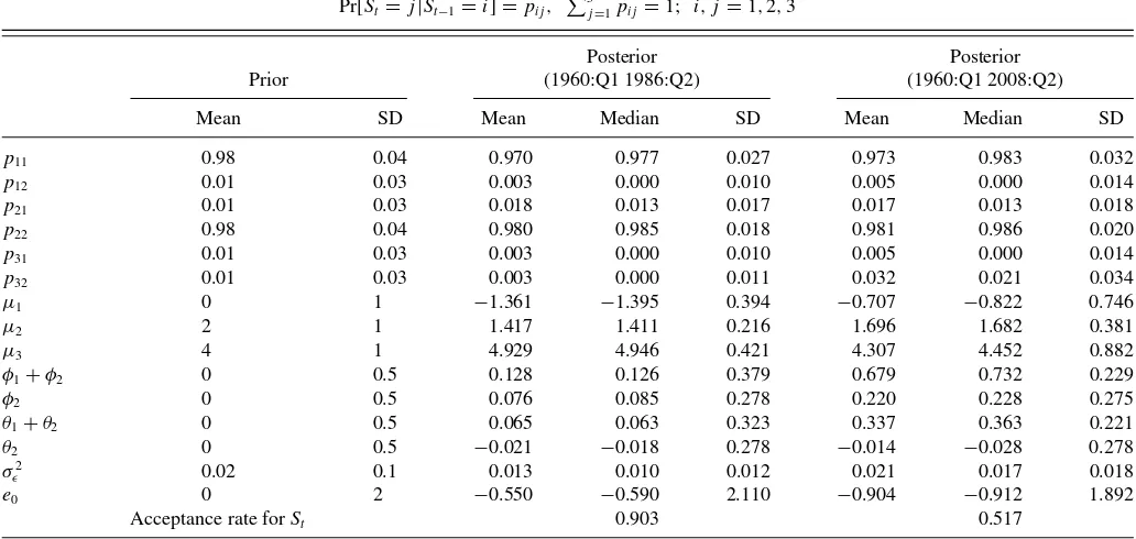
Table 3. Posterior moments: AR (2) model with Markov-switching mean (Garcia and Perron1996)
rEP
t =µSt+φ1(rtEP−1−µSt−1)+φ2(rtEP−2−µSt−2)+et
et ∼N(0, σt2)
ln(σ2
t)=ln(σt2−1)+ωt, ωt ∼N(0, σω2)
Pr[St =j|St−1=i]=pij,
3
j=1pij =1; i, j=1,2,3
Posterior Posterior
Prior (1960:Q1 1986:Q2) (1960:Q1 2008:Q2)
Mean SD Mean Median SD Mean Median SD
p11 0.98 0.04 0.970 0.977 0.027 0.973 0.983 0.032
p12 0.01 0.03 0.003 0.000 0.010 0.005 0.000 0.014
p21 0.01 0.03 0.018 0.013 0.017 0.017 0.013 0.018
p22 0.98 0.04 0.980 0.985 0.018 0.981 0.986 0.020
p31 0.01 0.03 0.003 0.000 0.010 0.005 0.000 0.014
p32 0.01 0.03 0.003 0.000 0.011 0.032 0.021 0.034
µ1 0 1 −1.361 −1.395 0.394 −0.707 −0.822 0.746
µ2 2 1 1.417 1.411 0.216 1.696 1.682 0.381
µ3 4 1 4.929 4.946 0.421 4.307 4.452 0.882
φ1+φ2 0 0.5 0.128 0.126 0.379 0.679 0.732 0.229
φ2 0 0.5 0.076 0.085 0.278 0.220 0.228 0.275
θ1+θ2 0 0.5 0.065 0.063 0.323 0.337 0.363 0.221 θ2 0 0.5 −0.021 −0.018 0.278 −0.014 −0.028 0.278 σ2
ǫ 0.02 0.1 0.013 0.010 0.012 0.021 0.017 0.018
e0 0 2 −0.550 −0.590 2.110 −0.904 −0.912 1.892
Acceptance rate forSt 0.903 0.517
NOTES: 1. Burn-in/total iterations = 5000/25,000. 2. SD refers to standard deviation.
3. A highest posterior density (HPD) region is a posterior density interval, the narrowest one possible with a chosen probability.
Figure 2. Posterior distribution of sum of AR coefficients: ARMA (2,2) and AR(2) models with Markov-switching mean (1960:Q1– 2008:Q2). Dotted line is for AR(2) and solid line for ARMA(2,2).
EARR. We performed white-noise tests for the standardized prediction errors and their squares, as implied by the AR(2) model for EPRR. Even though we could not reject the null that they are white-noise processes for the Garcia and Perron sample, the null was rejected at a 5% significance level for the extended sample. This evidence suggests that an AR(2) model with a Markov-switching mean for the EPRR is misspecified for an extended sample period of 1960Q1–2008Q2.
When moving average (MA) terms are included for the Garcia and Perron sample (1960Q1–1986Q2), the posterior moments of the parameters reported inTable 3suggest that the results are almost the same as in the case of Garcia and Perron’s (1996) AR(2) model. The posterior mean of the sum of AR coeffi-cients, as well as that of the sum of MA coefficoeffi-cients, is close to zero. For the extended sample (1960Q1–2008Q2), however, the dynamics of the EARR implied by our ARMA(2,2) model are drastically different from those for an AR(2) model of Garcia and Perron (1996). The posterior median of the sum of AR coef-ficients is 0.732, with the 90% highest posterior density (HPD) being [0.299,0.999]. Note that the posterior median of the AR coefficient sum in an AR(2) model is only 0.330 the 90% highest posterior Density (HPD) being [0.125,0.550]. If we compare the posterior distribution of the sum of AR coefficients for an AR(2) model and that for our ARMA(2,2) model depicted inFigure 2, the difference in the persistence dynamics of the EARR as im-plied by the two model are clearer. That is, omitting MA terms in the model of EPRR considerably underestimates the persistence of the EARR for the extended sample.
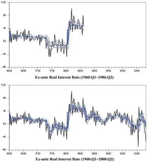
The plot of the EARR in the lower panel ofFigure 3shows that the EARR varies considerably within each regime, in contrast to the conclusion of Garcia and Perron (1996). Furthermore, when we performed diagnostic checks for our ARMA(2,2) model, we could not reject the null hypothesis that the standardized prediction errors and their squares are white-noise processes.
6. SUMMARY AND CONCLUSION
In this article, we provide an efficient MCMC algorithm for making inference of regime-switching ARMA models, by em-ploying a multi-move sampler when sampling the state variables
Figure 3. Ex-ante real rate: ARMA (2,2) model with Markov-switching mean (proposed model).
from the proposal distribution. As discussed by Liu, Wong, and Kong (1994) and Scott (2002), one potential weakness of the al-gorithm based on a single-move sampler is that, its performance gets worse with slower mixing as the persistence of the latent state variable increases. However, our simulation study in Sec-tion4shows that the proposed algorithm based on a multi-move sampler achieves reasonably fast convergence to the posterior distribution, even when the latent regime-indicator variable is highly persistent or even when there exist absorbing states.
We apply the proposed model and the algorithm to U.S. data on EPRR, to investigate the dynamics of the latent EARR under regime shifts. The rational expectations assumption implies the EPRR follows an ARMA process, if we assume that the latent EARR follows an AR process. We argue Garcia and Perron’s (1996) conclusion that the EARR rate is a constant subject to occasional jumps may be sample-specific. For an extended sam-ple that includes recent data, Garcia and Perron’s (1996) AR(2) model of EPRR may be misspecified, and we show that exclud-ing the theory-implied movexclud-ing-average terms may understate the persistence of the EARR dynamics. Our empirical results suggest that, even though we rule out the possibility of a unit root in the EARR, it may be more persistent and volatile than has been documented in some of the literature including Garcia and Perron (1996).
APPENDIX A: GENERATING ARMA PARAMETERS,ψ,
CONDITIONAL ON MS STATES, ˜ST
Recursive data transformation schemes developed by Chib and Greenberg (1994) are introduced in this section, which produces sim-ple linear regression relationships forµ, φ, ande0. They successfully
yield full conditional densities under a general ARMA(p, q) model and are employed for posterior Gibbs sampling. However, the
rior simulation ofθis complicating since its conditional posterior does not belong to standard families of distributions. Chib and Greenberg (1994) suggested employing an MH algorithm forθ to successfully implement their Bayesian approach. While they provided a proposal density function forθ, which requires an additional estimation step, we, instead, use a random-walk proposal density function. This particular class of MH algorithm with a random-walk density is referred to as a random-walk chain MH algorithm. (see Koop2003.) In the case of low acceptance probabilities, Chib and Greenberg’s (1994) algorithm can be employed as an alternative.
A.1 Generating Transition Probabilities Conditional on
˜
YT, ˜ST, and Other Parameters
Assuming an independent Dirichlet distribution for the prior of
Pi=[pi1 pi2 . . . piM]′, theith column of the matrix of the
transi-tion probabilities,P, we have:
Prior : Pi∼Dirichlet(ui1, ui2, . . . , ui,M),
Posterior : Pi|Y˜T,S˜T, −q ∼Dirichlet(ui1+ni1, ui2
+ni2, . . . , uiM+niM), (A.1)
whereuij forj=1,2, . . . , M, are known hyper parameters of the
priors;nijrefers to the number of the transitions from stateitojin ˜ST,
which can be easily counted.
A.2 GeneratingφConditional on ˜YT, ˜ST, and Other
Parameters−φ
The following is the necessary data transformation step for generat-ingφ:
The transformed data ¯Y and ¯X yield a desirable linear regression equation in terms ofφ, which is employed for constructing the follow-ing conventional normal posterior:
Prior : φ∼ N(φ, )Iφ,
whereφandare a prior mean and a prior variance, respectively;
Iφis an indication function for stationarity; ¯φ=¯(−1φ+σ−2X¯′Y¯)
First, we show recursive data transformations for generatingµ:
Y∗=X∗µ+e,
The generated datasets,Y∗andX∗have a conventional linear
re-gression relationship as well. Therefore, the prior and the posterior densities ofµare given by
Prior : µ∼N(µ, µ)Iµ,
whereµandµare a prior mean and a prior variance, respectively;
Iµ is the indication function for identification of MS regimes; ¯µ=
¯
a posterior mean and a posterior covariance matrix, respectively.
A.4 GeneratingθConditional on ˜YT, ˜ST, and Other
Parameters−θ
To generateθ, an MH algorithm is inevitable as the error term,et,
is not a linear function ofθ. Chib and Greenberg (1994) suggested a proposal density ofθbased on the first-order Taylor expansion and the nonlinear least-square estimation, which requires additional classical estimation and data transformation steps. We, instead, take advantage of a random-walk chain MH algorithm as an alternative to simplify these steps (see Koop2003). In the procedure, a candidate density is defined as
θ∗=θm−1+ε, (A.6) whereθ∗is a new candidate sample;θm−1is a previously acceptedθin
the previous MCMC iteration; andεis an increment random variable. The corresponding acceptance probability is given by
α(θ∗, θm−1)=min
that a choice for the density ofεcompletes the proposal density. We take a common choice ofε, which is a multi-variate normal with mean 0 and a variance-covariance, c. c is appropriately chosen to get
an acceptance probability between 0.2 and 0.5, which is the range advocated by Koop (2003).
The posterior simulation onθis conducted with the proposal gener-ating function in Equation (A.7). The prior and the posterior are given by
whereθ andθ are a prior mean and a prior variance, respectively;
Iθis the indication function for invertibility; ¯θand ¯θare a posterior
mean and a posterior variance;et(θ)=(yt−µSt)−φ(yt−1−µSt−1)− θ et−1=y¯t−x¯tφ=yt∗−x∗tµ, which can be obtained in the preceding
transformations.
A.5 Generatinge0Conditional on ˜YT, ˜ST, and Other
Parameters−e0
Chib and Greenberg (1994) proposed a method to estimatee0based
on the Kalman filter and the backward recursions with the Moore–
Penrose inverse. We follow an efficient alternative by Nakatsuma (2000) to avoid the complexity. The following is the required data transformation step that generates a simple linear regression equation in terms ofe0:
of the above data transformation can be verified by the fact thatet=
ˆ
yt−xˆte0.
The generated data have a conventional linear regression relationship conditional on−e0. Therefore, it is now straightforward to drawe0
from the following conditional posterior density:
Prior : e0∼N(e0, e0),
where e0 and e0 are a prior mean and a prior variance, respec-tively; ¯e0 and ¯e0 are a posterior mean and a posterior variance;
¯
The posterior simulation onσ2is straightforward given one of the
previously transformed datasets. The posterior samples onσ2are drawn
from the following conditional posterior density:
Prior : σ2∼IG
whereνandδare prior degrees of freedom and a prior scale parameter, respectively; ¯ν=ν+T; ¯δ=δ+d, whered=T calculated would lead to slightly different values ofd, this would not make significant differences on the Bayesian estimates. This step completes the MCMC algorithm of an ARMA (p, q) model with a Markov-switching mean conditional on ˜ST.
APPENDIX B. GENERATING ˜ST FROM THE
PROPOSED MULTI-MOVE PROPOSAL DENSITY
B.1 State-Space Representation of ARMA(p,q) Models
Consider the following general MS-ARMA (p, q) model:
yt =µSt +
(p, q) model are dependent uponMdiscrete unobserved states (St=
1,2, . . . , M) at each time period. We assume stationarity and invert-ibility under all regimes. The ARMA (p, q) model in Equation (B.1)
can be equivalently expressed as the following:
yt =µSt+ut,
Finally, Equation (B.2) has the following state-space representation:
Measurement Equation.
St are dependent upon an
unobserved, discrete-valued, M-state Markov-switching variable St
(St =1,2, . . . , M);Imis anm×midentity matrix. Transition
proba-bilities are given in Equation (2).
B.2 Conditional Kalman Filter
Here in the state-space model with Markov switching, we need to use the conventional Kalman filter conditional onSt−1=iandSt =j
However, notice that each iteration of the above Kalman filter pro-duces anM-fold increase in the number of cases to consider. For ex-ample,M10cases should be considered by the time,t= 10. As a result,
without some approximation, the above Kalman filter is not operable. Kim (1994) proposed an algorithm to complete the above Kalman fil-ter by collapsing (M×M) posteriors (α(t|i,jt ), Pt(|i,jt )) intoMposteriors (α(tj|t), P
(j) t|t ).
B.3 Approximated Filtering Algorithm by Kim (1994)
The approximated filtering algorithm by Kim (1994) is a combina-tion of the Kalman filter and the Hamilton filter, along with appropriate approximations. It starts with initial valuesα0(j|0),P
(j)
0|0, andf[S0], which
are the unconditional mean and covariance matrix of the unobserved process ofαtconditional on stateS0=jand the steady state
probabil-ity of the Markov chain process, respectively. The filtering algorithm contains the following steps:
1. Run the Kalman filter given in Equations (B.5)– (B.10) fori, j=
1,2, . . . , Mto get the followings:
α(ti,j|t−)1, Pt(|i,jt−)1, η(ti,j|t−)1, ft(|i,jt−)1, α(ti,j|t ), Pt(|i,jt ).. (B.11)
2. Calculate Pr[St =j|Y˜t] forj=1,2, . . . , Mthrough the following
Hamilton filter:
f(St, St−1|Y˜t−1)=f(St|St−1)f(St−1|Y˜t−1) (B.12)
f(yt|Y˜t−1)=
St
St−1
f(yt|Y˜t−1, St, St−1)f(St, St−1|Y˜t−1)
(B.13)
f(St, St−1|Y˜t)=
f(yt, St, St−1|Y˜t−1) f(yt|Y˜t−1)
= f(yt|St, St−1,
˜
Yt−1)f(St, St−1|Y˜t−1) f(yt|Y˜t−1)
(B.14)
Pr[St =j|Y˜t]=
St−1
f(St =j, St−1|Y˜t). (B.15)
3. Using the conditional probabilities from the Hamilton filter, collapse
M×Mposteriors in Equations (B.9) and (B.10) intoMposteriors using the following approximations:
α(tj|t) ≈
St−1f
St =j, St−1 Y˜t
α(ti,j|t )
PrSt =j
Y˜t
(B.16)
Pt(|jt) ≈
St−1f
St=j, St−1 Y˜t
Pt(|i,jt )+αt(j|t)−α(ti,j|t )
αt(j|t)−αt(i,j|t )
Pr[St =j|Y˜t]
. (B.17)
4. Repeat Steps 1–3 and save approximated Pr[St=j|Y˜t] for j=
1,2, . . . , Min each iteration for Bayesian inference on ˜ST.
The resulting Pr[St =j|Y˜t],j=1,2, . . . , M for t = 1,2,...,T with
the above approximations is used ash(St|Y˜t) for the proposal density
function in Equation (13).
ACKNOWLEDGMENTS
Chang-Jin Kim acknowledges financial support from the National Research Foundation of Korea Grant funded by the Korean Government (NRF-R1303501 and KRF-2008-342-B00006) and from the Bryan C. Cressey Professorship at the University of Washington. An earlier version of this article has been included as Chapter 2 of Jaeho Kim’s Ph.D. dissertation at the University of Washington. Jaeho Kim acknowledges the support of the Grover and Creta Ensley Fellowship in Economic Policy from the University of Washington.
[Received November 2013. Revised September 2014.]
REFERENCES
Albert, J. H., and Chib, S. (1993), “Bayes Inference via Gibbs Sampling of Autoregressive Time Series Subject to Markov Mean and Variance Shifts,” Journal of Business and Economic Statistics, 11, 1–15. [568]
Antoncic, M. (1986), “High and Volatile Real Interest Rates: Where Does the Fed Fit In?,”Journal of Money, Credit, and Banking, 18, 18–27. [566] Bai, J., and Perron, P. (2003), “Computation and Analysis of Multiple Structural
Change Models,”Journal of Applied Econometrics, 18, 1–22. [566] Bauwens, L., Dufays, A., and Rombouts, J. (2014), “Marginal Likelihood for
Markov-Switching and Change-Point GARCH,”Journal of Econometrics, 178, 508–522. [567]
Billio, M., Casarin, R., and Osuntuy, A. (in press), “Efficient Gibbs Sampling for Markov Switching GARCH Models,”Computational Statistics and Data Analysis. [567]
Billio, M., Monfort, A., and Robert, C. P. (1999), “Bayesian Estimation of Switching ARMA Models,”Journal of Econometrics, 93, 229–255. [567,568,569,570,571]
Caporale, T., and Grier, K. B. (2000), “Political Regime Change and the Real Interest Rate,” Journal of Money, Credit, and Banking, 32, 320–334. [566]
Carter, C. K., and Kohn, P. (1994), “On Gibbs Sampling for State Space Models,” Biometrica, 81, 541–553. [567]
Chib, S. (1998), “Estimation and Comparison of Multiple Change-Point Mod-els,”Journal of Econometrics, 86, 221–241. [568]
Chib, S., and Greenberg, E. (1994), “Bayes Inference in Regression Mod-els With ARMA(p, q) Errors,” Journal of Econometrics, 64, 183–206. [567,568,574,575]
——— (1995), “Understanding the Metropolis-Hastings Algorithm,” The American Statistician, 49, 327–335. [568]
Cosslett, S. R., and Lee, L.-F. (1985), “Serial Correlation in Latent Discrete Variable Models,”Journal of Econometrics, 27, 79–97. [569]
Crowder, W. J., and Hoffman, D. L. (1996), “The Long-Run Relationship Be-tween Nominal Interest Rates and Inflation: The Fisher Equation Revisited,” Journal of Money, Credit, and Banking, 28, 102–118. [566]
De Jong, P., and Shephard, N. (1995), “The Simulation Smoother for Time Series Models,”Biometrika, 82, 339–350. [567]
Diebolt, J., and Robert, C. P. (1994), “Estimation of Finite Mixture Distributions by Bayesian Sampling,”Journal of the Royal Statistical Society, Series B, 56, 363–365. [569]
Fama, E. F. (1975), “Short-Term Interest Rates as Predictors of Inflation,” American Economic Review, 63, 269–282. [566]
Fiorentini, G., Planas, C., and Rossi, A. (2012), “Efficient MCMC Sampling in Dynamic Mixture Models,”Statistics and Computing, 27, 1–13. [567] Fruehwirth-Schnatter, S. (2006),Mixture and Markov-Switching Models, New
York: Springer. [567]
Gali, J. (1992), “How Well Does the IS-LM Model Fit Postwar U.S. Data?,” Quarterly Journal of Economics, 107, 709–738. [566]
Garbade, K., and Wachtel, P. (1978), “Time Variation in the Relationship Be-tween Inflation and Interest Rates,”Journal of Monetary Economics, 4, 755–765. [566]
Garcia, R., and Perron, P. (1996), “An Analysis of the Real Interest Rate Under Regime Shifts,”Review of Economics and Statistics, 78, 111–125. [566,567,569,571,572,574]
Geweke, J. (1992), “Evaluating the Accuracy of Sampling-Based Approaches to the Calculation of Posterior Moments,”Bayesian Statistics, 4, 169–193. [571]
Gilks, W. R., Richardson, S., and Spiegelhalter, D. J. (1996), “Introducing Markov Chain Monte Carlo,” inMarkov Chain Monte Carlo in Practice, eds. W. R. Gilks and D. J. Spiegelhalter, US: Springer, pp. 1–19. [568] Hamilton, J. D. (1988), “Rational Expectations Econometric Analysis of
Changes in Regimes: An Investigation of the Term Structure of Interest Rates,”Journal of Economic Dynamics and Control, 12, 385–432. [569] ——— (1989), “A New Approach to the Economic Analysis of Nonstationary
Time Series and the Business Cycle,”Econometrica, 57, 357–384. [569] Harrison, P. J., and Stevens, C. F. (1976), “Bayesian Forecasting,”Journal of
the Royal Statistical Society, Series B, 38, 205–247. [569]
Huizinga, J., and Mishkin, F. S. (1986), “Monetary Regime Shifts and the Unusual Behavior of Real Interest Rates,”Carnegie-Rochester Conference Series on Public Policy, 24, 231–274. [566]
Kim, C.-J. (1994), “Dynamic Linear Models With Markov-Switching,”Journal of Econometrics, 60, 1–22. [567,568,569,570,577]
Kim, S., Shepard, N., and Chib, S. (1998), “Stochastic Volatility: Likelihood In-ference and Comparison With ARCH Models,”Review of Economic Studies, 65, 361–393. [572]
King, R. G., Plosser, C. I., Stock, J. H., and Watson, M. W. (1991), “Stochastic Trends and Economic Fluctuations,”American Economic Review, 81, 819– 840. [566]
Koop, G. (2003),Bayesian Econometrics, New York: Wiley. [568,575] Koustas, Z., and Serletis, A. (1999), “On the Fisher Effect,”Journal of Monetary
Economics, 44, 105–130. [566]
Liu, J. S., Wong, W. H., and Kong, A. (1994), “Covariance Structure of the Gibbs Sampler With Applications to the Comparisons of Estimators and Augmentation Schemes,”Biometrika, 81, 27–40. [567,569,574]
Mishkin, F. S. (1981), “The Real Rate of Interest: An Empirical Investigation,” CarnegieRochester Conference Series on Public Policy, 15, 151–200. [566] ——— (1992), “Is the Fisher Effect for Real? A Reexamination of the Relation-ship Between Inflation and Interest Rates,”Journal of Monetary Economics, 30, 195–215. [566]
Nakatsuma, T. (2000), “Bayesian Analysis of ARMA-GARCH Models: A Markov Chain Sampling Approach,”Journal of Econometrics, 95, 57–69. [567,568,576]
Neely, C. J., and Rapach, D. E. (2008), “Real Interest Rate Persistence: Evidence and Implications,” Working Paper 2008-018A, Federal Reserve Bank, St. Louis. [566]
Nelson, C. R., and Schwert, G. W. (1977), “Short-Term Interest Rates as Predictors of Inflation: On Testing the Hypothesis That the Real Interest Rate is Constant,” American Economic Review, 67, 478–486. [566]
Perron, P. (1990), “Testing for a Unit Root in a Time Series with a Chang-ing Mean,”Journal of Business and Economic Statistics, 8, 153–162. [566]
Rapach, D. E., and Weber, C. E. (2004), “Are Real Interest Rates Really Non-stationary? New Evidence From Tests With Good Size and Power,”Journal of Macroeconomics, 26, 409–430. [566]
Rose, A. K. (1988), “Is the Real Interest Rate Stable?,”Journal of Finance, 43, 1095–1112. [566]
Scott, S. L. (2002), “Bayesian Methods for Hidden Markov Models: Recur-sive Computing in the 21st Century,”Journal of the American Statistical Association, 97, 337–351. [567,569,574]
Shephard, N. (1994), “Partial Non-Gaussian State Space,”Biometrika, 81, 115– 131. [567]
Sun, Y., and Phillips, C. B. P. (2004), “Understanding the Fisher Equation,” Journal of Applied Econometrics, 19, 869–886. [566]