Full Terms & Conditions of access and use can be found at
http://www.tandfonline.com/action/journalInformation?journalCode=ubes20
Download by: [Universitas Maritim Raja Ali Haji] Date: 12 January 2016, At: 23:56
Journal of Business & Economic Statistics
ISSN: 0735-0015 (Print) 1537-2707 (Online) Journal homepage: http://www.tandfonline.com/loi/ubes20
Panel Stationarity Tests for Purchasing Power
Parity With Cross-Sectional Dependence
David Harris, Stephen Leybourne & Brendan McCabe
To cite this article: David Harris, Stephen Leybourne & Brendan McCabe (2005) Panel
Stationarity Tests for Purchasing Power Parity With Cross-Sectional Dependence, Journal of Business & Economic Statistics, 23:4, 395-409, DOI: 10.1198/073500105000000090
To link to this article: http://dx.doi.org/10.1198/073500105000000090
View supplementary material
Published online: 01 Jan 2012.
Submit your article to this journal
Article views: 96
View related articles
Panel Stationarity Tests for Purchasing Power
Parity With Cross-Sectional Dependence
David H
ARRISDepartment of Economics, University of Melbourne, Victoria 3010, Australia (harrisd@unimelb.edu.au)
Stephen L
EYBOURNESchool of Economics, University of Nottingham, Nottingham NG7 2RD, U.K. (steve.leybourne@nottingham.ac.uk)
Brendan M
CC
ABESchool of Management, University of Liverpool, Liverpool L69 7ZH, U.K. (Brendan.McCabe@liv.ac.uk)
We investigate the purchasing power parity (PPP) hypothesis for a group of 17 countries using a new panel-based test of stationarity that allows for arbitrary cross-sectional dependence. We treat the short-run time series dynamics nonparametrically and thus avoid the need to fit separate, and potentially misspeci-fied, models for the individual series. The statistic is simple to compute and uses standard normal critical values, even in the presence of a wide range of different deterministic components. We also evaluate the behavior of the test using a factor model to approximate cross-sectional dependence and find that it generally improves finite-sample performance. Taken together, these features provide a widely applicable solution to the problem of testing for stationarity versus unit roots in macro-panel data. The test finds sig-nificant evidence against the PPP null hypothesis being true, even when allowance is made for structural breaks.
KEY WORDS: Cross section; Dependence; Factor model; Panel data; PPP; Stationarity tests; Time series.
1. INTRODUCTION
Relatively long time series of many core macroeconomic variables are now available for most developed economies. The use of panel data, in particular unit root or stationarity tests, to empirically validate various important macroeconomic theories has become a rapid growth area of applied econo-metric research. For example, panel tests have been used to assess the evidence for the hypotheses of purchasing power par-ity (PPP), for convergence of growth rates, for mean reversion of inflation rates, and for the real interest rate parity hypoth-esis. These tests attempt to exploit the potential power gains offered by analyzing a time series panel as opposed to indi-vidual series, and as such, they have the potential to provide more compelling evidence for or against certain models of eco-nomic behavior. Recent tests have been proposed by, inter alia, O’Connell (1998), Maddala and Wu (1999), Hadri (2000), Choi (2001, 2002), Chang and Song (2002), Levin, Lin, and Chu (2002), Shin and Snell (2002), Chang (2004), and Im, Pesaran, and Shin (2003).
One of the major factors that any panel test needs to be able to address if reliable inference is to be made in prac-tical situations is cross-sectional dependence. Cross-sectional dependencies are likely to be the rule rather than the excep-tion in studying cross-country data, because the existence of strong intereconomy linkages, and this is particularly true in the context of testing PPP. The tests of Hadri (2000), Choi (2001), Levin et al. (2002), Shin and Snell (2002), and Im et al. (2003) all assume independence across the panel, and their size properties are suspect when this rather unrealistic assumption does not hold. The test of O’Connell (1998) al-lows for cross-sectional dependence, but this is restricted to the innovation term driving an assumed common auto-regressive (AR) process in the model. The method of Choi (2002) permits
cross-sectional dependence, but only after imposing a com-mon additive error component across the panel. The testing ap-proach adopted by Chang and Song (2002) provides, at least in theory, a general treatment of the problem of cross-sectional dependence, but their procedure relies on user-supplied para-meters, whose values are a function of the dependence structure itself, which rather limits its practical appeal. Maddala and Wu (1999) and Chang (2004) approached the problem indirectly, relying on bootstrap procedures, but the underlying tests are not pivotal. Regarding time series dynamics, with the excep-tion of the test of Hadri (2000), all of these tests rely on fitting an appropriately specified time series regression model to each individual series in the panel (a tedious and error-prone under-taking unless the cross-sectional dimension is relatively small). For tests that allow cross-sectional dependence, this is a doubly vital requirement, because any notion of these tests’ robustness to cross-sectional dependence is intimately reliant on the cor-rect modeling of the time series dynamics.
Recently, Bai and Ng (2004a,b) suggested using a fac-tor model to account for cross-sectional dependence in panel data. Their idea is to orthogonally decompose a panel of time series into a fixed number of independent common fac-tors and remaining idiosyncratic components that are indepen-dent (or weakly depenindepen-dent). Bai and Ng (2004a,b) constructed Dickey–Fuller and Kwiatkowski, Phillips, Schmidt, and Shin (1992; KPSS) tests for estimates of the unobserved compo-nents, although they did not explicitly provide tests for the ob-served series. Although the performance of the Dickey–Fuller
© 2005 American Statistical Association Journal of Business & Economic Statistics October 2005, Vol. 23, No. 4 DOI 10.1198/073500105000000090
395
approach may be deemed satisfactory, that of the KPSS proce-dure is much less so, because of significant problems with the size of the tests.
It would seem, then, that none of the extant approaches of-fers a totally satisfactory solution to the problem of testing for stationarity when the cross-sectional dependence structure and time series dynamics are both unknown. In contrast, the new stationarity test statistic that we suggest in this article is constructed so as to overcome both these problems. We allow for arbitrary unknown cross-sectional dependence between the series in the panel; the series may be contemporaneously or cross-serially dependent. We also permit a wide range of het-erogeneous stationary time series dynamics, which includes the conventional autoregressive moving average (ARMA) class.
Our statistic is based on a vector version of the stationar-ity test of Harris, McCabe, and Leybourne (2003) (hereinafter HML) rather than on a KPSS-type stationarity test like that Hadri (2000). The statistic is, in essence, the sum of the lag-k sample autocovariances across the panel, suitably studentized, where we allow k to be a simple increasing function of the time dimension. By controlling k in such a way, we remove any need to explicitly model the time series dynamics of each series in the panel, even though their time series dynamics may be quite heterogeneous. At the same time, the studenti-zation automatically robustifies the statistic to the presence of any form of cross-sectional dependence. The statistic is simple to construct and, conveniently, has a limiting null distribution that is standard normal under quite general linear process as-sumptions. Asymptotics are based on a fixed cross-sectional di-mension, and passing the time series dimension to infinity. For many macroeconomic applications, however, we believe that the assumption of a fixed cross-section dimension appears rea-sonable. Asymptotic normality also holds when the statistic is calculated using residuals from deterministic regression models fitted to each series. These may include polynomial trends or even structural breaks and there is no requirement that the same deterministic model be fitted to each series. As such, the test can be applied across a range of empirically relevant modeling situ-ations without reference to model-dependent null critical values or the need to compute bootstrap critical values. We also show how our new statistic can be applied to a factor model. The test when applied to an estimated factor model can have signifi-cantly more power than the test applied to the raw data. The same is true even if the factor model is misspecified. We also show how to construct a pooled KPSS test for the observed se-ries in the factor model and compare its performance with our new panel stationarity tests by means of some Monte Carlo ex-periments.
After the simulations, we reassess the evidence for PPP in a panel of 17 U.S. dollar real exchange rate series from 1973–1998 using our new tests. The validity of the PPP hy-pothesis has attracted a vast amount of attention in recent times and has been tested extensively using different panel unit root tests. In general, little evidence in support of PPP has been uncovered. For example, O’Connell (1998), Maddala and Wu (1999), Cheung and Lai (2000), and Chang and Song (2002) were unable to provide convincing evidence against the unit root null. In fact, what limited empirical evidence there is in support of PPP has arisen mainly from application of tests that
do not account for cross-sectional dependence at all (see, e.g., Oh 1996; Wu 1996). More recently, Wu and Wu (2001) and Papell (2002) found some evidence for PPP, after accounting for cross-correlation using bootstrap methods. However, even when a rejection of the unit root null is found, this cannot be interpreted as evidence for PPP holding in the entire panel, be-cause it may be that only a subset of the real exchange rates are stationary. In view of this, it makes some sense to apply our panel stationarity test. Here the PPP hypothesis is represented by the null of panel stationarity, and a rejection can then, ce-teris paribus, fairly unambiguously be interpreted as evidence against the PPP hypothesis being true. To counter the possi-bility that the episodic behavior of the dollar during the 1980s may unduly disguise the existence of PPP, we also allow for de-terministic structural breaks in each series, thus paralleling the approach of Papell (2002). We find that our preferred test still rejects the PPP hypothesis very strongly.
The plan of the article is as follows. In the next section we introduce our statistic by explaining how it can be used to dis-tinguish between stationarity and unit roots in the panel con-text. We also derive its asymptotic properties and show how to incorporate deterministic regression effects. In Section 3 we show how our test may be applied to the observed series in the context of Bai and Ng’s (2004a) factor model. We also demon-strate how a KPSS test may be constructed for the observed data. In Section 4 we report the results of a number of Monte Carlo experiments to gauge the empirical size and power of the tests. The results are very encouraging. In particular, the robust-ness of the new panel stationarity test’s size to different patterns of cross-sectional dependence and time series dynamics stands out as a prominent characteristic. In addition, significant power gains are available by using the new statistic in combination with Bai and Ng’s (2004a) estimated factor model. We provide details of the PPP application in Section 5, and give a summary in Section 6.
2. A PANEL TEST OF STATIONARITY WITH
CROSS–SECTIONAL CORRELATION
Consider a panel ofNtime series {zi,t,t=1, . . . ,T}
gener-ated by the processes
zi,t=φizi,t−1+ζi,t, i=1,2, . . . ,N,t=1,2, . . . ,T, (1)
where each mean-0 disturbance term,{ζi,t,t=1, . . . ,T}isI(0)
andζi,t andζj,t may be correlated for anyiandj. Throughout,
we considerN fixed and letT grow in our limit theory. It is possible to allow the number of observations to vary with the individual time series involved, but we use a singleTfor nota-tional convenience. We wish to test the null hypothesis of joint stationarity,
H0:|φi|<1 for alli,
against the unit root alternative,
H1:φi=1 for at least onei.
2.1 Motivation
To motivate our statistic, fixiand suppose for simplicity that {ζi,t,t=1, . . . ,T}in (1) is iid with variance σi2, and
follow-ing section 2.1 of HML, consider a test statistic for the vari-ablezi,t based on the scaled first-order sample autocovariance
Ci,1=T−1/2Tt=2zi,tzi,t−1. Suitably centered and studentized, this is the Dickey–Fuller statistic for testing the null hypoth-esis φi=1. But for testing H0:|φi|<1, the difficulty is that
E(Ci,1)≃T1/2σi2φi/(1−φi2), so that the null distribution
de-pends onφi. We instead consider the correspondingkth-order
autocovariance,
shown in section 5 of HML thatCi,kis asymptotically standard
normal when suitably studentized, and hence any dependence of the null distribution onφi(andσi2) is removed. Whenφi=1,
E(Ci,k)≃T3/2σi2, and it can be shown the studentized statistic
is divergent. Hence, for a singlezi,t, a consistent test with
stan-dard normal asymptotic null distribution can be based onCi,k
withk→ ∞.
To construct a joint test ofH0:|φi|<1 for alli, we follow the
literature on panel Dickey–Fuller tests and consider the sum of the individual test statistics,
simultaneously. In factCk, when suitably studentized, has an
asymptotic standard normal distribution underH0. UnderH1, suppose without loss of generality thatφi=1 fori=1, . . . ,sN so that the leading right-side term once more suggests that the test should be consistent.
2.2 The Test Statistic and Its Distribution Theory
We assume that ζt =(ζ1,t, . . . , ζN,t)′ follows the
station-ary linear process assumption (assumption LP) of HML. This assumption permits cross-sectional correlation of any form between the series in the panel; this correlation may be contem-poraneous or cross-serial. In addition, it allows for heterogene-ity in the dynamics and variation across the panel. The series may exhibit a range of individual temporal dependence struc-tures, including those of stationary ARMA processes.
Definingak,t=Ni=1zi,tzi,t−k, the statisticCkcan be written
Written in this way, the statisticSk can be seen to be the
stan-dardized mean of the constructed seriesak,tdivided by its
long-run standard deviation, which provides some intuition for the following result.
Lemma 1. If the conditions of theorems FCLT and LRV of HML hold for ζt andk=O(T1/2)then, as T→ ∞(with Nfixed), the following results hold:
(a) Sk⇒N[0,1]underH0.
(b) Skdiverges to+∞underH1.
This lemma is a special case of Theorem 1 (Sec. 2.3), and so its proof is omitted. Theorems FCLT and LRV of HML impose conditions on the choice ofkandl, the truncation parameter of the LRV. In this article we require thatk= [(δT)1/2]for some constantδ >0 and l/k→0 asT→ ∞. (Here[·]denotes the integer part of the argument.)
The role of the appropriate specification of kand ωˆ2{ak,t}
is to remove the effects of the temporal dependence in in-dividual series from the asymptotic null distribution of Sk.
Because Sk depends on zi,t andzi,t−k only through the
cross-sectional sum ak,t=Ni=1zi,tzi,t−k, any valid estimate of the
long-run variance of {ak,t}will automatically correct for any
pattern of cross-sectional dependence in zi,t. Hence there is
no need to parametrically model the dynamic structure of each series or their cross-sectional dependencies. A similar LRV approach was adopted by Driscoll and Kraay (1998) to generalized method-of-moments (GMM) inference for panel data with cross-sectional dependence but without the added complication ofk→ ∞.
2.3 Deterministic Regression Effects
The statisticSk is generally not feasible, because in practice
eachzi,twill be estimated from a regression on some
determin-istic terms. Such vectors of determindetermin-istics are denoted byxi,t
and may be different for eachiif required. In place of (1), we consider the model given by
yi,t=βi′xi,t+zi,t, zi,t=φizi,t−1+ζi,t,
i=1,2, . . . ,N,t=1,2, . . . ,T. (3)
Letzˆi,tdenote an ordinary least squares (OLS) residual from the
regression (3), that is,zˆi,t=yi,t− ˆβi′xi,t, whereβˆi is the usual
OLS estimator. It is desirable that the statistic be invariant to
relative rescaling of the series, so in place ofzi,tin the definition
ofSk, we instead use the standardized residuals
˜
zi,t= ˆzi,t/si, (4)
wheresi is the sample standard deviation ofˆzi,t. The resulting
statistic is
It can be shown that Sˆk has an asymptotic standard
nor-mal null distribution, and when dealing with a snor-mall number of series, this often proves to be an adequate approximation for the finite-sample distribution. But if the panel dimension is not relatively small, then individual finite-sample errors that arise from the estimation of the regression models combine in the construction of the aggregate numerator C˜k =Ni=1C˜i,k
and can significantly affect the finite-sample null distribution of Sˆk. To see how this arises, write the numerator of Sˆk as
˜
Ck =Ni=1C˜i,k, where C˜i,k =T−1/2Tt=k+1z˜i,t˜zi,t−k. After
some manipulation,C˜i,kmay be expressed as
˜
The first term in this expression is asymptotically normal un-der the null, and the effect of the regression estimation er-ror is captured by (5). Under H0, the term in square brackets in (5) isOp(1), and so the whole term isOp(T−1/2). Because
the term (5) is clearly negative, it induces a negative finite-sample error into each individual statistic and the amplification of this problem is obvious when we subsequently considerC˜i,k
summed overN. Because we are conducting upper-tail tests, ce-teris paribus, the effect of this is toreducethe finite-sample size of the test. It is possible to produce a finite-sample correction for this regression estimation error by subtracting an estimate of the term (5) fromC˜i,k. It is shown in the proof of Theorem 1
that the expectation of the term in square brackets in (5) can be consistently estimated by
This is the usual matrix version of the scalar long-run vari-anceωˆ{·}2. Specializing to the case of a constant,xi,t=1, we
can compute c˜i = ˆω2{˜zit} and in the case of xi,t= [1,wi,t]′,
˜
ci= ˆω2{˜zit} + ˆω2{˜zitw˜i,t}, wherew˜i,t=(wi,t− ¯wi)/sw,iandsw,i
is the standard deviation of the variablewi,t.
To summarize, our recommended statistic for application is
˜
the following theorem is given in the Appendix.
Theorem 1. If the conditions of theorem RES of HML hold for ζt,xi,t in (3), and k= [δT]1/2 (for some constant δ >0),
then, asT→ ∞(withNfixed), the following results hold:
(a) S˜k⇒N[0,1]underH0.
(b) S˜kdiverges to+∞underH1.
Theorem RES of HML specifies quite general conditions onxi,t, allowing for a wide range of deterministic regression
functions including constants, linear and polynomial trends, dummy variables, structural breaks, and various other models. The theorem shows that a consistent test is obtained by reject-ingH0for values ofS˜k greater than the appropriate upper-tail
critical value from the standard normal distribution. As a prac-tical matter, we implement the test in Sections 4 and 5 using l= [12(T/100)1/4]inωˆ2{˜ak,t}andk= [(3T)1/2].
3. PANEL TESTS FOR STATIONARITY IN
FACTOR MODELS
An alternative approach to panel stationarity testing in the presence of cross-sectional correlation is based on the factor model of Bai and Ng (2004a,b). Instead of the nonparametric model (1), consider the factor model
yi,t=βi′xi,t+zi,t, (9)
zi,t=λ′ift+ei,t, (10)
whereftis anr×1 vector of latent factors,λiis anr×1 vector
of loading parameters, and ei,t is an idiosyncratic component
for eachi. It is assumed thatft=(f1,t, . . . ,fr,t)′andei,tsatisfy iandj. The null hypothesis for the panel stationarity test based on (9)–(12) is
H′0:|αj|<1,|ρi|<1 for alli,j,
against the alternative hypothesis
H′1:αj=1 for at least onejand/orρi=1 for at least onei.
Our testS˜kapplied to the estimates of the cross-correlated zi,t
generated by (9)–(12) has its usual asymptotic properties, that
is, a standard normal limit distribution underH0′ and divergence to+∞underH1′. We may also consider, however, a variant of this test that is applied instead to estimates of the uncorrelated componentsfj,t andei,t. The intuition here is that when a
para-metric form of cross-correlation is present, there might be po-tential gains, not least in terms of finite-sample test power, by removing it before constructing the test, as opposed to effec-tively ignoring its presence.
Bai and Ng (2004a) gave a detailed explanation of how to estimaterand the unobserved componentsfj,tandei,tvia
prin-cipal components analysis, an approach that we summarize as part of Appendix A.2. They constructed unit root tests for the estimated components, and also Bai and Ng (2004b) provided stationarity tests based on the well-known univariate stationar-ity test of Kwiatkowski, Phillips, Schmidt, and Shin (1992). By testing the unit root or stationarity properties of the estimated components rather than the observable series, Bai and Ng were able to sidestep the problems arising from cross-correlations among series and to deduce detailed information about the time series properties of the panel. In this article, however, as we deal with a single test for the null hypothesis that the series {zi,t,t=1, . . . ,T}are stationary for all i, our approach is to
apply S˜k to all of the estimated components jointly.
Specifi-cally, letfˆj,t,j=1, . . . ,rˆ, andeˆi,t,i=1, . . . ,N, denote the
esti-mated components, and letf˜j,t ande˜i,t denote the same
com-ponents standardized to have unit variance. The statistic (8) can then be calculated from the estimated components by re-defining ˜zi,t to be the ith element of the (N+ ˆr)×1 vector
(˜f1,t, . . . ,f˜ˆr,t,˜e1,t, . . . ,e˜N,t)′. We denote the resulting statistic
byS˜Fk.
To yield consistent estimates of r, fj,t, and ei,t under H0′ andH1′, Bai and Ng required that both T andN approach in-finity. Recall that in this article we considerN fixed, and as a result, ˆr, ˆfj,t, and eˆi,t are not consistent estimators in this
context. This, it turns out, does not preventS˜kFfrom being as-ymptotically (asT→ ∞ withN fixed) normal under the null and divergent under the alternative. The reason for this stems from the fact that our original statisticS˜khas asymptotic
prop-erties that do not depend, under either the null or the alternative, on the pattern of cross-correlation present in the observed data from which it is constructed. Because the estimatesfˆj,tandeˆi,t
are, asymptotically (inT withN fixed) nothing more than lin-ear transformations of the originalyi,t, it follows that Theorem 1
applies toS˜Fk, which is simplyS˜kcalculated from the
(standard-ized)fˆj,tandeˆi,t. Note that because of the principal components
method used to construct the factors, underH0′, thefˆj,t andeˆi,t
remainI(0)and underH1′ still containI(1)components. Hence ˜
SkFhas the same asymptotic properties underH0′ andH′1and the conditions of Theorem 2 asS˜kin Theorem 1. In regard to
finite-sample properties, however, the inconsistency of theˆfj,tandeˆi,t
obviously does not precludeS˜kFfrom having potentially better finite-sample properties thanS˜k. Our finite-sample simulations
in Section 4 do indeed reveal thatS˜Fk often has superior finite-sample power.
Bai and Ng’s factor model estimation considers only the cases wherexi,tin (9) contains a constant or linear trend term
(and hence does not depend oni). Clearly, allowance for a more flexible deterministic component is again worthwhile, not in
the least because the model in Section 5 involves deterministic trend functions allowing structural breaks whose dates differ across i. We provide, in Appendix A.2, full details of estima-tion of the factors(fˆ1,t, . . . ,fˆrˆ,t,eˆ1,t, . . . ,ˆeN,t)and computation
ofS˜Fk when the factor model is extended to permit general de-terministic terms.
Theorem 2. If the conditions of theorem RES of HML hold for(ut,vt)andxi,tandk= [δT]1/2(for some constantδ >0),
then, asT→ ∞(withNfixed), the following results hold:
(a) S˜Fk ⇒N[0,1]underH0′. (b) S˜Fk diverges to+∞underH′1.
Thus, in common with S˜k, a consistent test is obtained by
rejectingH′0for values ofS˜Fk greater than the appropriate upper-tail critical value from the standard normal distribution.
3.1 A KPSS Test for the Estimated Components
A point of comparison for theS˜Fk andS˜ktests is provided by
a simple adaptation of the pooled KPSS stationarity test of Bai and Ng (2004b). It is also a variation of the approach of Hadri (2000), where the pooled KPSS stationarity test was applied directly toyi,tassuming no cross-sectional correlation. The
in-dividual KPSS statistics for the estimated components are
ηfF,j=T
Theµsubscript denotes the inclusion of a intercept only in (9). Herecˆ1,T andcˆ2,T are constants whose values are taken from
Table 1. We obtain these by generating 2,000 realizations from (9)–(12) with βi=ρi=r=0, so thatzi,t∼iid N[0,1]for all
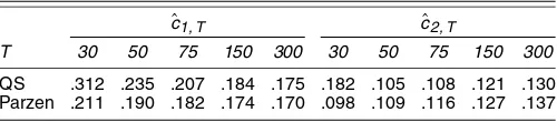
i and t. In calculating ωˆ2{·}, the Parzen and quadratic spec-tral (QS) lag windows with bandwidthl= [12(T/100)]1/4were used (following Yin and Wu 2000 and Bai and Ng 2004b). For each combination of sample sizesNandT, constants were com-puted from the means and standard deviations of the sampling distributions ofη¯Fµ. The constants demonstrate substantial vari-ation withT, but very little variation over the values ofN con-sidered here.
It follows from theorem 1 of Bai and Ng (2004b) and the-orem 1 of Hadri (2000) that η¯Fµ has an asymptotic standard
Table 1. Finite-Sample Constants for theη¯µStatistic
ˆ
c1, T cˆ2, T
T 30 50 75 150 300 30 50 75 150 300
QS .312 .235 .207 .184 .175 .182 .105 .108 .121 .130 Parzen .211 .190 .182 .174 .170 .098 .109 .116 .127 .137
normal distribution under H′0 as N and T approach infinity. Under H1′, those individual statistics corresponding to nonsta-tionary components diverge to+∞, so the test rejectsH0when
¯
ηFµ is larger than the appropriate upper-tail critical value from the standard normal distribution.
In principle, theη¯Fµtest could be extended to allow general deterministic regression of the form (9), but in practice this would be difficult, because it would require the computation of further constants. For example, if structural breaks were to be included, then the constants would depend on the number of breaks and the break dates. As a result of this difficulty, and also because of the inferior finite-sample performance of theη¯Fµtest reported in Section 4, we do not pursue the pooled KPSS ap-proach in our PPP application given in Section 5.
A theoretical difference between testing viaS˜k (orS˜Fk) and
¯
ηFµ is that S˜k and S˜Fk use an asymptotic approximation with
T→ ∞andNfixed, whereasη¯µFuses bothT andN approach-ing infinity. The requirement thatN→ ∞is important for the consistent estimation of the common factors and idiosyncratic components in model (9) and, although this is relevant toη¯µF, it is not a consideration forS˜korS˜Fk. Compared withS˜kandS˜Fk,
we believe that the η¯Fµ test is less robust because of the pos-sibility in practice for underspecifying the factor model, that is, including an insufficient number of factors in the estimated model, leading to inconsistent estimation. We include simula-tions in Section 4 that clearly demonstrate the finite-sample ef-fects of factor underspecification on the behavior of η¯Fµ. Note that S˜Fk remains valid in the presence of such underspecifica-tion, because Theorem 1 still applies.
4. FINITE–SAMPLE PROPERTIES
In this section we report the results of a simulation experi-ment to evaluate the finite-sample properties of the three tests considered in this article. To our knowledge, no other existing panel test for stationarity that is valid in the presence of cross-sectional correlation can be included in the experiment. As a benchmark, however, we also simulate the standard, nonfactor version of the Hadri (2000) test, denoted by η¯µ. Each test
in-cludes a constant term in the deterministic specification. The data-generating process is the factor model (9)–(12), withβi=0, and with disturbances(u1,t, . . . ,ur,t,v1,t, . . . ,vN,t)′
drawn from the N[0,Ir+N]distribution. The number of factors
included arer=0,2 and 7. There is no cross-sectional depen-dence whenr=0. Whenr=2,7, we considerλi∼iid N[κ, κ2]
(fixed across replications) withκ=3, which is the same as used by Bai and Ng (2004b) except for the multiplicative constantκ. Estimation of the factor model is implemented assuming a max-imum number of common factors ofrmax=6 when choosing the number of factors. So the estimated factor model may be specified correctly when r=0 or 2, but it is always misspec-ified when r=7. We include the r=7 case purely to give some indication of the consequences of misspecifying the fac-tor model (which in practice could be due to underspecification of the number of factors or to a model with a fixed number of factors being inappropriate). Becauseuj,tandvi,tare both
stan-dard normal variates,κ is used to control the relative standard deviations of the factors compared with the idiosyncratic com-ponents. The value ofκ turns out to be unimportant forr=2
but is important forr=7 when the factor model is misspeci-fied, because it determines the relative magnitude of the factor that is omitted. The choice ofκ=3 is within the range of em-pirical standard deviation ratios reported in table 4 of Bai and Ng (2004b) for a panel of quarterly real exchange rates. Pre-dictably, unreported simulations reveal that the consequences of model misspecification are worse whenκis increased from 3 and better whenκ is decreased.
Under the simulation data-generating process, the model (9)–(12) can be represented in the form of (1), and vectorized as
yt=yt−1+ζt,
whereyt=(y1,t, . . . ,yN,t)′ and is a diagonal matrix with
elementsφi. Hereζthas some covariance matrix, say. In the
situation whereφi=φfor alli, we have
−1/2yt=φ−1/2yt−1+−1/2ζt,
and hence−1/2ythas a diagonal covariance matrix. Consider
applying S˜k (the other tests can be treated similarly) to both
ytand−1/2yt. This allows us to gauge howS˜kdeals on its own
with cross-correlation, as opposed to this correlation being han-dled by a known generalized least squares (GLS) transforma-tion−1/2yt. Of course, applying S˜k to the GLS-transformed
data is the same as just applying the test to uncorrelated data in the first place. Thus we simply need to compare simulations results forS˜k when r>0 (which implies that is
nondiago-nal) to those whenr=0 ( is diagonal). Note that ifφi =φ
for alli(as in some of our size simulations and all of our power simulations), then the transformed data−1/2yt do not have
a diagonal covariance matrix, and so such a comparison is no longer meaningful.
The sample sizes that we consider areN=10,20,30,40 and T =30,50,75,150,300, which we chose to include realistic sample sizes for macroeconometric applications. After prelim-inary experimentation, we implement the S˜k andS˜Fk statistics
usingk= [(3T)1/2]and estimate the long-run variances using a Bartlett lag window withl= [12(T/100)1/4]. Following Bai and Ng (2004b), we compute the long-run variances forη¯Fµ us-ing the QS lag window withl= [12(T/100)1/4]. Unreported simulations showed that the Parzen lag window suggested by Yin and Wu (2000) for the test of Hadri (2000) is inferior to the QS lag window in this case. All experiments are based on 5,000 replications, and all tests are taken to reject the null hy-pothesis at the 5% significance level when the test statistic is larger than 1.65.
4.1 Size of Tests
Under the null hypothesis, the values ofαj andρi in (11)
and (12) considered are(αj, ρi)=(0,0),(.4,0),(.8,0),(0, .4),
(0, .8)for alliandj. Hence any difference in the effect of au-tocorrelation in the factors and idiosyncratic components can be evaluated. We also considerαj andρidrawn independently
from a U[0, .8]distribution for alliandj(fixed across replica-tions) to include some heterogeneity across the components.
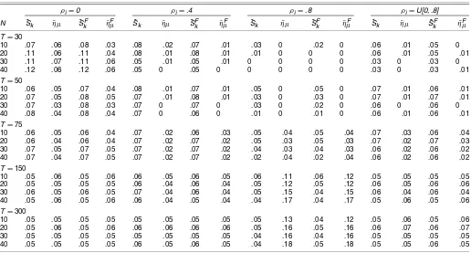
Table 2 contains estimated finite-sample sizes forr=0; the case of no cross-sectional dependence. Throughout,S˜k andS˜Fk
behave very similarly, as doη¯µandη¯µF. The results forρi=0
reveal actual sizes near the asymptotic .05 level. The only ex-ception is some mild oversizing for the S˜k and S˜Fk tests for
T=30, although it is not surprising that an asymptotic approx-imation based on T → ∞ with N fixed is not very accurate whenT is small andN is about the same magnitude. Increas-ing ρi to introduce idiosyncratic autocorrelation reveals that
˜
Sk andS˜Fk are well behaved for ρi=.4 and somewhat
under-sized for smallT andρi=.8. Theη¯µandη¯Fµ tests are
under-sized forρi=.4 and smallT, whereas they are oversized when
ρi=.8, even withT=300.
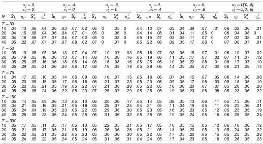
Table 3 gives the results for the cross-correlated case where r=2. HereS˜k has reasonably good size control everywhere,
as doesS˜kFoutside ofT=30. Interestingly, forS˜Fk, strong auto-correlation in the common factors does not lead to small-sample undersizing in the same way as it does in the idiosyncratic com-ponents. As might be expected, η¯µ controls size poorly,
be-ing generally quite oversized. The factor versionη¯Fµ performs somewhat better but is still oversized in the presence of strong autocorrelation. For the reasons noted earlier, apart from the cases where theαj or ρi are generated as heterogeneous
uni-form variates, the results of Table 3 can be compared with those forS˜kandη¯µin Table 2, which are effectively the GLS
bench-marks of test performance. It then becomes clear that unless T is small, the size properties ofS˜k,S˜Fk, andη¯µF in Table 3 do
not differ in any deleterious manner from those of S˜k andη¯µ
calculated using an exact (but in practice infeasible) GLS trans-formation.
Finally, Table 4 gives the results for r=7. The proper-ties of S˜k are essentially the same as for r=2. So too are
those of S˜Fk, though there is now no longer any evidence of small-sample undersizing when the autocorrelation in the idiosyncratic components is high. This nicely illustrates the ro-bustness to cross-correlation of both tests, together with
robust-ness to factor model underspecification of the latter test. A point of interest is the performance ofη¯Fµ here, because it relies on the correct specification of the model. Across all values of the AR parameters, it is clear thatη¯Fµbecomes progressively over-sized asT increases. In fact, apart from the small values ofT, its pattern of oversizing is quite similar to that of its nonfactor counterpart,η¯µ. This shows that factor model misspecification
can have rather serious consequences forη¯Fµ.
In summary, then, in regard to finite-sample size properties, it is clear that S˜k andS˜Fk both behave well across a range of
processes generating different patterns of cross-sectional de-pendence and autocorrelation. Of the two, S˜k is marginally
preferable because its performance with very small samples, although any differences quickly become negligible as the sam-ple sizes increase toward levels most typically encountered with macroeconomic data.
4.2 Power of Tests
In the alternative hypotheses that we consider, we setρi=1
fori=1, . . . ,sNandρi=0 fori=sN+1, . . . ,N, wheres≤.6.
Forr=2, we setα1=1,α2=0 andα1=1,α2=1. We also consider hybrid alternatives where unit roots appear simulta-neously in the idiosyncratic and factor components. Analysis involvingη¯µis not generally included, because, as seen earlier,
its size control is very poor in the presence of cross-correlation. Similarly, we do not include results for r=7, because the model for computing η¯Fµ is misspecified, which again results in poor size control.
Table 5 first reports powers for the non–cross-correlated case wherer=0, so that power arises from unit roots in the idiosyn-cratic components alone. The results forS˜kandS˜Fk reveal power
Table 2. Simulated Size: r=0
ρi=0 ρi=.4 ρi=.8 ρi=U[0, .8]
N S˜k η¯µ S˜Fk η¯µF S˜k η¯µ S˜Fk η¯µF S˜k η¯µ S˜kF η¯µF S˜k η¯µ S˜Fk η¯Fµ
T=30
10 .07 .06 .08 .03 .08 .02 .07 .01 .03 0 .02 0 .06 .01 .05 0
20 .11 .06 .11 .04 .08 .01 .08 .01 .01 0 0 0 .06 .01 .05 .01
30 .11 .07 .11 .06 .05 .01 .05 .01 0 0 0 0 .03 0 .03 0
40 .12 .06 .12 .06 .05 0 .05 0 0 0 0 0 .03 0 .03 .01
T=50
10 .06 .05 .07 .04 .08 .01 .07 .01 .05 0 .05 0 .07 .01 .06 .01
20 .07 .05 .08 .05 .07 .01 .08 .01 .03 0 .03 0 .07 .01 .07 .01
30 .07 .03 .08 .03 .07 0 .07 0 .03 0 .02 0 .06 0 .06 0
40 .08 .04 .08 .04 .07 0 .06 0 .01 0 .01 0 .06 .01 .06 .01
T=75
10 .06 .05 .06 .04 .07 .02 .06 .03 .05 .04 .05 .04 .07 .03 .06 .04
20 .06 .04 .06 .04 .07 .02 .07 .02 .05 .03 .05 .03 .07 .02 .07 .03
30 .07 .05 .07 .05 .07 .02 .07 .02 .04 .03 .04 .03 .06 .02 .06 .02
40 .07 .04 .07 .05 .07 .02 .07 .02 .02 .04 .02 .04 .06 .02 .06 .02
T=150
10 .05 .06 .05 .06 .06 .05 .06 .05 .06 .11 .06 .12 .05 .05 .05 .05
20 .05 .05 .05 .05 .06 .04 .06 .04 .05 .12 .05 .12 .06 .05 .06 .06
30 .06 .05 .06 .05 .07 .04 .06 .04 .05 .15 .04 .15 .06 .04 .06 .04
40 .05 .06 .05 .06 .06 .04 .05 .04 .04 .17 .04 .17 .05 .06 .05 .06
T=300
10 .05 .05 .05 .05 .05 .05 .05 .05 .05 .13 .04 .12 .05 .06 .05 .06
20 .05 .06 .05 .06 .06 .06 .06 .06 .05 .16 .05 .16 .06 .07 .06 .07
30 .05 .05 .05 .05 .05 .05 .05 .05 .04 .16 .04 .16 .05 .05 .05 .05
40 .05 .05 .05 .05 .06 .05 .06 .05 .04 .18 .05 .18 .05 .05 .06 .05
Table 3. Simulated Size: r=2
αj=0, αj=.4, αj=.8, αj=0, αj=0, αj=U[0, .8], ρi=0 ρi=0 ρi=0 ρi=.4 ρi=.8 ρi=U[0, .8] N S˜k η¯µ S˜kF η¯Fµ S˜k η¯µ S˜Fk η¯µF S˜k η¯µ S˜kF η¯µF S˜k η¯µ S˜kF η¯Fµ S˜k η¯µ S˜Fk η¯Fµ S˜k η¯µ S˜Fk η¯Fµ
T=30
10 .03 .13 .08 .03 .05 .06 .08 .02 .08 .01 .07 .01 .04 .10 .07 .01 .06 .04 .03 0 .05 .09 .06 .01 20 .03 .17 .10 .03 .05 .08 .09 .02 .08 .01 .07 .01 .04 .15 .06 .01 .05 .07 .01 0 .05 .08 .05 .01 30 .03 .21 .10 .03 .06 .10 .09 .02 .07 .02 .07 .01 .03 .20 .05 0 .04 .10 0 0 .06 .08 .03 0 40 .03 .23 .11 .03 .05 .11 .09 .02 .07 .02 .07 0 .03 .21 .05 0 .05 .09 0 0 .05 .11 .03 0 T=50
10 .04 .22 .07 .04 .05 .17 .06 .03 .07 .16 .07 .05 .04 .20 .07 .01 .05 .09 .06 .01 .05 .17 .07 .01 20 .04 .27 .08 .03 .05 .21 .08 .03 .08 .20 .08 .05 .05 .23 .08 .01 .06 .13 .03 0 .06 .19 .06 0 30 .04 .27 .08 .02 .05 .21 .08 .02 .07 .19 .07 .05 .04 .26 .07 0 .05 .16 .02 0 .05 .22 .05 0 40 .05 .31 .08 .03 .06 .25 .08 .03 .08 .23 .08 .06 .05 .29 .06 0 .06 .16 .01 0 .06 .24 .05 0 T=75
10 .05 .19 .06 .05 .05 .17 .07 .05 .07 .21 .07 .09 .05 .16 .06 .04 .05 .10 .07 .05 .05 .17 .07 .04 20 .05 .25 .06 .04 .05 .24 .06 .04 .07 .26 .07 .12 .04 .24 .07 .02 .04 .18 .04 .03 .05 .21 .06 .02 30 .05 .26 .07 .03 .05 .25 .06 .04 .07 .29 .07 .13 .05 .24 .07 .01 .05 .18 .03 .03 .05 .23 .06 .02 40 .04 .30 .08 .04 .05 .28 .07 .05 .07 .32 .08 .17 .05 .29 .07 .01 .05 .24 .02 .03 .05 .25 .06 .02 T=150
10 .06 .18 .05 .06 .06 .18 .05 .06 .06 .24 .06 .12 .05 .17 .06 .05 .05 .13 .06 .10 .05 .17 .06 .08 20 .05 .24 .06 .05 .05 .24 .05 .05 .06 .31 .05 .15 .05 .23 .06 .05 .05 .20 .05 .12 .05 .23 .05 .07 30 .05 .27 .05 .05 .05 .27 .06 .05 .05 .33 .05 .15 .04 .25 .06 .04 .05 .22 .05 .13 .05 .25 .05 .06 40 .05 .28 .05 .04 .05 .28 .06 .05 .06 .34 .05 .17 .05 .27 .05 .03 .05 .25 .04 .15 .06 .32 .05 .07 T=300
10 .05 .20 .05 .06 .05 .21 .05 .06 .05 .26 .05 .11 .05 .19 .05 .06 .05 .16 .04 .12 .05 .22 .05 .08 20 .05 .24 .05 .06 .05 .26 .05 .06 .06 .31 .05 .13 .05 .23 .06 .06 .05 .19 .05 .15 .05 .25 .05 .08 30 .05 .24 .05 .05 .05 .25 .05 .05 .05 .30 .05 .12 .05 .23 .05 .05 .05 .20 .05 .15 .05 .26 .05 .07 40 .05 .27 .05 .05 .05 .27 .05 .05 .06 .34 .06 .13 .04 .25 .05 .05 .04 .23 .04 .15 .05 .31 .05 .08
increasing with T, as expected, and, interestingly, power also generally increasing withN. Throughout, the powers ofS˜kand
˜
SFk are very similar, apart from whenN=10, in which caseS˜Fk has a modest advantage in smaller samples. The pattern of re-sults is qualitatively similar forη¯µandη¯Fµ, although the power
advantage of η¯Fµ over η¯µ when N=10 is more pronounced.
Outside ofN=10, we find thatS˜kandS˜Fk are generally a good
deal more powerful thanη¯µandη¯Fµ. As Table 2 shows, the sizes
of all four tests forρi=0 are very similar forT>30, and the
superior power ofS˜kandS˜Fk is not simply artifactual.
Table 4. Simulated Size: r=7
αj=0, αj=.4, αj=.8, αj=0, αj=0, αj=U[0, .8], ρi=0 ρi=0 ρi=0 ρi=.4 ρi=.8 ρi=U[0, .8] N S˜k η¯µ S˜kF η¯Fµ S˜k η¯µ S˜Fk η¯µF S˜k η¯µ S˜Fk η¯µF S˜k η¯µ S˜Fk η¯µF S˜k η¯µ S˜Fk η¯Fµ S˜k η¯µ S˜Fk η¯Fµ
T=30
10 .04 .13 .06 .04 .06 .03 .07 .02 .06 0 .05 0 .04 .10 .07 .03 .04 .09 .07 .01 .06 .02 .06 .01 20 .04 .15 .08 .04 .06 .04 .07 .01 .05 0 .06 0 .04 .14 .08 .01 .04 .11 .05 0 .06 .04 .08 0 30 .04 .16 .06 .07 .07 .04 .07 .02 .05 0 .08 0 .05 .15 .07 .03 .05 .11 .07 0 .07 .02 .08 .01 40 .05 .22 .07 .07 .07 .07 .08 .02 .07 0 .07 0 .05 .22 .08 .02 .05 .17 .06 0 .07 .08 .07 .01 T=50
10 .05 .19 .06 .05 .06 .13 .07 .04 .07 .10 .07 .03 .05 .18 .07 .03 .05 .15 .07 .01 .06 .10 .07 .02 20 .05 .19 .05 .16 .06 .13 .07 .14 .08 .10 .08 .16 .05 .19 .06 .11 .05 .17 .07 .02 .07 .11 .07 .12 30 .05 .25 .05 .16 .06 .18 .06 .14 .08 .16 .08 .16 .05 .25 .06 .10 .05 .22 .08 .01 .06 .17 .07 .10 40 .05 .29 .05 .21 .06 .20 .06 .17 .08 .16 .08 .19 .05 .28 .06 .14 .05 .25 .07 .02 .06 .21 .08 .14 T=75
10 .04 .17 .05 .10 .05 .14 .06 .09 .06 .16 .07 .15 .05 .16 .06 .07 .04 .15 .07 .05 .06 .14 .06 .08 20 .05 .20 .05 .15 .05 .17 .06 .16 .06 .21 .07 .23 .05 .20 .06 .09 .05 .17 .06 .03 .05 .18 .05 .10 30 .05 .22 .05 .21 .05 .19 .05 .22 .07 .21 .08 .28 .05 .22 .05 .16 .06 .20 .07 .07 .05 .20 .06 .20 40 .05 .26 .05 .24 .06 .22 .05 .23 .07 .25 .07 .29 .05 .25 .05 .19 .05 .23 .06 .08 .05 .23 .06 .22 T=150
10 .05 .14 .05 .09 .06 .13 .05 .10 .06 .20 .06 .17 .05 .14 .05 .08 .05 .13 .06 .11 .05 .13 .06 .11 20 .04 .21 .05 .16 .05 .21 .05 .18 .05 .28 .07 .25 .04 .21 .05 .11 .04 .19 .05 .11 .05 .23 .06 .21 30 .05 .24 .04 .19 .05 .23 .05 .22 .05 .29 .06 .30 .05 .23 .05 .16 .05 .23 .05 .12 .05 .23 .05 .19 40 .05 .25 .05 .23 .06 .24 .05 .25 .06 .31 .06 .32 .05 .25 .05 .19 .05 .24 .05 .16 .06 .25 .05 .24 T=300
10 .05 .17 .05 .11 .05 .17 .05 .13 .05 .22 .05 .21 .05 .17 .05 .10 .05 .15 .05 .12 .06 .16 .06 .12 20 .05 .21 .05 .17 .05 .21 .05 .19 .06 .26 .06 .26 .05 .21 .05 .13 .05 .20 .05 .13 .05 .24 .05 .22 30 .05 .22 .05 .21 .05 .22 .05 .23 .05 .30 .06 .30 .05 .22 .05 .17 .05 .20 .05 .15 .05 .25 .05 .26 40 .05 .24 .05 .22 .05 .24 .05 .24 .05 .31 .06 .31 .04 .24 .05 .17 .04 .23 .05 .16 .05 .26 .05 .23
Table 5. Simulated Power: r=0
s=.1 s=.2 s=.4 s=.6
N S˜k η¯µ S˜kF η¯Fµ S˜k η¯µ S˜kF η¯µF S˜k η¯µ S˜Fk η¯µF S˜k η¯µ S˜kF η¯Fµ
T=30
10 .15 .05 .20 .01 .18 .04 .25 .01 .24 .03 .27 0 .28 .02 .26 0
20 .18 .05 .18 .03 .21 .04 .20 .02 .25 .02 .25 .01 .28 .02 .26 .01
30 .17 .06 .16 .04 .20 .04 .19 .03 .24 .03 .23 .02 .27 .02 .25 .02
40 .17 .05 .17 .05 .21 .04 .20 .04 .25 .03 .24 .02 .27 .01 .26 .01
T=50
10 .18 .06 .31 .33 .28 .08 .44 .42 .47 .17 .57 .47 .60 .32 .65 .48
20 .22 .08 .22 .08 .35 .12 .35 .13 .60 .29 .60 .29 .76 .51 .75 .51
30 .25 .07 .25 .06 .42 .11 .42 .12 .70 .31 .70 .31 .86 .58 .86 .58
40 .28 .09 .28 .09 .48 .17 .47 .17 .76 .46 .76 .46 .90 .77 .90 .77
T=75
10 .22 .11 .36 .45 .37 .20 .55 .67 .65 .50 .75 .82 .82 .76 .84 .89
20 .30 .14 .30 .14 .55 .32 .55 .32 .84 .72 .84 .72 .95 .94 .95 .94
30 .35 .16 .35 .16 .65 .41 .65 .41 .93 .87 .93 .87 .99 .99 .99 .99
40 .43 .21 .43 .21 .73 .54 .73 .54 .97 .95 .97 .95 1.00 1.00 1.00 1.00
T=150
10 .39 .24 .40 .26 .68 .50 .71 .61 .93 .88 .94 .96 .99 .98 .99 .99
20 .56 .36 .56 .36 .88 .75 .88 .75 .99 .98 .99 .98 1.00 1.00 1.00 1.00
30 .67 .43 .67 .43 .96 .87 .96 .87 1.00 .99 1.00 .99 1.00 1.00 1.00 1.00
40 .79 .53 .79 .53 .98 .93 .98 .93 1.00 1.00 1.00 1.00 1.00 1.00 1.00 1.00
T=300
10 .66 .47 .66 .47 .91 .80 .91 .80 .99 .98 .99 .98 1.00 1.00 1.00 1.00
20 .86 .65 .86 .65 .99 .95 .99 .95 1.00 .99 1.00 .99 1.00 1.00 1.00 1.00
30 .94 .77 .94 .77 1.00 .98 1.00 .98 1.00 1.00 1.00 1.00 1.00 1.00 1.00 1.00
40 .98 .82 .98 .82 1.00 .99 1.00 .99 1.00 1.00 1.00 1.00 1.00 1.00 1.00 1.00
Table 6 induces cross-correlation withr=2. Hereη¯µnow is
not included. In the first two parts of Table 6, both factors are stationary (noise), so the unit roots arise only in the idiosyn-cratic components. By some way, the most striking feature of this part of the table is the large drop in the power ofS˜krelative
toS˜Fk. Other than this, we also see that for the smaller values ofT,S˜Fk remains more powerful thanη¯Fµ; however, there is now little to choose from between them for the larger values ofT.
In the next three parts of Table 6, the first common factor contains a unit root, whereas the second common factor is
sta-Table 6. Simulated Power: r=2
s=.2, s=.6, s=0, s=.2, s=.6, s=0, s=.2, s=.6, α1=0, α1=0, α1=1.0, α1=1.0, α1=1.0, α1=1.0, α1=1.0, α1=1.0, α2=0 α2=0 α2=0 α2=0 α2=0 α2=1.0 α2=1.0 α2=1.0 N S˜k S˜Fk η¯µF S˜k S˜kF η¯Fµ S˜k S˜kF η¯Fµ S˜k S˜kF η¯µF S˜k S˜kF η¯Fµ S˜k S˜kF η¯µF S˜k S˜Fk η¯µF S˜k S˜kF η¯Fµ
T=30
10 .06 .24 0 .12 .25 0 .22 .20 .01 .23 .26 0 .23 .26 0 .28 .25 0 .28 .27 0 .28 .26 0 20 .08 .21 .01 .12 .24 0 .26 .23 .01 .26 .26 0 .27 .25 0 .29 .25 0 .29 .27 0 .30 .25 0 30 .05 .19 .01 .11 .19 0 .26 .23 .01 .26 .25 .01 .26 .22 0 .29 .26 0 .30 .27 0 .30 .23 0 40 .05 .18 .01 .11 .20 0 .27 .24 0 .27 .25 0 .28 .22 0 .31 .27 0 .31 .26 0 .31 .22 0 T=50
10 .07 .44 .41 .18 .63 .44 .38 .31 .36 .38 .52 .44 .40 .67 .47 .45 .41 .42 .45 .58 .45 .46 .71 .47 20 .09 .44 .32 .18 .79 .57 .37 .35 .42 .40 .55 .51 .41 .82 .65 .45 .48 .52 .46 .66 .56 .47 .87 .66 30 .07 .51 .35 .14 .85 .63 .35 .35 .44 .36 .58 .52 .37 .88 .71 .46 .49 .55 .46 .67 .59 .47 .91 .73 40 .08 .53 .39 .18 .90 .72 .36 .36 .48 .37 .61 .59 .40 .92 .79 .48 .50 .61 .49 .70 .67 .50 .94 .83 T=75
10 .09 .60 .74 .38 .84 .89 .49 .42 .57 .50 .71 .82 .54 .88 .91 .61 .57 .70 .61 .78 .86 .64 .90 .91 20 .08 .70 .74 .21 .97 .97 .45 .45 .59 .46 .78 .85 .49 .97 .97 .58 .63 .77 .58 .86 .90 .58 .99 .98 30 .09 .78 .78 .33 .98 .98 .45 .44 .61 .45 .83 .88 .50 .99 .99 .58 .63 .78 .58 .89 .91 .60 1.00 1.00 40 .09 .83 .84 .32 .99 .98 .44 .45 .62 .45 .85 .09 .51 0 1.00 .59 .64 .80 .60 .90 .93 .61 1.00 1.00 T=150
10 .26 .84 .88 .77 .98 .98 .66 .60 .70 .68 .93 .95 .76 .99 .99 .82 .80 .87 .83 .96 .96 .84 1.00 1.00 20 .21 .94 .95 .79 .99 .99 .64 .62 .75 .66 .99 .99 .72 1.00 1.00 .83 .82 .90 .84 .99 .99 .85 1.00 1.00 30 .22 .98 .98 .79 1.00 1.00 .63 .62 .75 .64 .99 .99 .70 1.00 1.00 .83 .85 .91 .83 1.00 1.00 .85 1.00 1.00 40 .24 .99 .99 .84 1.00 1.00 .65 .64 .78 .67 .99 .99 .72 1.00 1.00 .82 .85 .92 .83 1.00 1.00 .84 1.00 1.00 T=300
10 .62 .96 .96 .99 1.00 1.00 .84 .82 .85 .86 .99 .99 .90 1.00 1.00 .96 .96 .96 .97 1.00 1.00 .97 1.00 1.00 20 .59 .99 .99 1.00 1.00 1.00 .84 .83 .87 .86 1.00 1.00 .91 1.00 1.00 .96 .97 .97 .96 1.00 1.00 .97 1.00 1.00 30 .46 1.00 1.00 1.00 1.00 1.00 .83 .82 .88 .83 1.00 1.00 .88 1.00 1.00 .95 .97 .97 .96 1.00 1.00 .97 1.00 1.00 40 .50 1.00 1.00 1.00 1.00 1.00 .83 .82 .88 .84 1.00 1.00 .92 1.00 1.00 .95 .97 .98 .96 1.00 1.00 .96 1.00 1.00
tionary. For s=0, unit roots arise only from this first factor; otherwise, fors>0, they also arise from the idiosyncratic com-ponents. Whens=0, the powers ofS˜kF andS˜kare again very
similar, but lower than those of η¯µF unless T=30. Fors=.2 ands=.6, the powers ofS˜Fk andη¯Fµare largely comparable for T>30, and now both are once more a good deal higher thanS˜k.
The final three parts of Table 6 repeat this analysis but with both common factors containing unit roots. Largely the same comments apply as made in the preceding paragraph, but with all tests demonstrating a modest rise in power.
Overall, then, the evidence from our size and power simula-tions would seem to confirm S˜Fk as the best compromise test. First, theS˜Fk test has only slightly poorer size properties thanS˜k
in the presence of cross-correlation. ButS˜kyields substantially
lower power thanS˜Fk in the presence of idiosyncratic unit roots combined with correlation—even when the factor cross-correlation is present in the stationary components alone. Sec-ond, although in certain situations theη¯Fµtest can appear more powerful thanS˜Fk, it has comparatively poor size control in the presence of strongly autocorrelated idiosyncratic components and is also highly susceptible to factor model misspecification.
5. TESTING THE PURCHASING POWER
PARITY HYPOTHESIS
In this section we empirically test the PPP hypothesis, which implies mean reversion (or stationarity) of bilateral real ex-change rates. We consider monthly real exex-change rates against the U.S. dollar for the following countries: Austria, Belgium, Canada, Denmark, Finland, France, Germany, Greece, Italy, Japan, Netherlands, Norway, Portugal, Spain, Sweden, Switzer-land, and the U.K. The real exchange rate data were constructed from raw nominal exchange rate and consumer price index data taken from the IMF International Financial Statistics database. It covers the period of the recent float, 1973.01–1998.12. We haveN=17 andT=312. In our notation we takeyi,tto be the
natural log of the real exchange rate, each standardized to have unit standard deviation.
5.1 Tests Allowing a Constant
As is standard in most PPP analysis, we first hypothesize that yi,thas a constant mean represented by
yi,t=µi+zi,t,
where the null hypothesis of PPP requires thatzi,t isI(0)and
the alternative hypothesis is thatzi,tisI(1). TheS˜ktest statistics
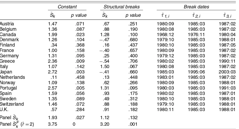
for each of the 17 series individually (i.e., each test is calculated withN=1) are given in Table 7 under the “Constant” heading, together with thepvalue of each test. At the .05 and .10 levels, the null hypothesis is rejected for 4 and 10 countries, so the evidence against PPP is mixed.
The panel S˜k statistic pooled across the 17 countries gives
˜
Sk=1.93 (p=.027). Estimation of the factor model (9)–(12)
for these data givesˆr=2 whenrmax=6, and the resulting test statistic isS˜Fk =3.75 (p=0). Thus both panel stationarity tests clearly reject the null hypothesis of PPP.
5.2 Tests Allowing Structural Breaks
Papell (2002) suggested that rejections of PPP in models that assume a constant mean can be explained by an unusual one-off episode in the 1980s, when there was a large unexplained appreciation of the U.S. dollar, followed by an equally large offsetting depreciation. In econometric terms, this translates to a generalization of the deterministic specification so that
yi,t=µi,t+zi,t, (14)
where
µi,t=
β1,i, t≤τ1,i
β2,i+β3,it, τ1,i≤t≤τ2,i
β4,i+β5,it, τ2,i≤t≤τ3,i
β1,i, τ3,i≤t,
(15)
and all of theβj,iandτj,imust be estimated. Papell (2002)
sug-gested that PPP holds around a constant long-run real exchange rate before breakpointτ1,i and after breakpointτ3,i. Note that
the same mean,β1,i, applies in these two time periods, and that
Table 7. PPP Tests
Constant Structural breaks Break dates
˜
Sk p value S˜k p value τˆ1, i τˆ2, i τˆ3, i
Austria 1.47 .071 .67 .251 1980:09 1985:03 1987:02
Belgium 1.36 .087 .88 .190 1980:08 1985:03 1987:02
Canada 1.99 .023 1.28 .100 1968:12 1976:11 1980:04
Denmark 1.26 .104 −.47 .680 1979:10 1985:03 1988:01
Finland .34 .368 .16 .437 1980:10 1985:03 1987:05
France 1.00 .158 −.40 .657 1980:09 1985:03 1987:02
Germany 1.31 .095 .25 .400 1979:12 1985:03 1987:02
Greece 2.36 .009 −.54 .706 1980:02 1985:03 1990:11
Italy 1.07 .142 1.50 .067 1980:08 1985:03 1987:02
Japan 2.72 .003 −.41 .660 1985:03 1995:06 2003:03
Netherlands .11 .458 .13 .448 1983:01 1985:03 1987:02
Norway 1.09 .138 .62 .266 1980:09 1985:03 1988:01
Portugal 2.57 .005 1.31 .095 1980:03 1985:03 1991:03
Spain 1.59 .056 .93 .175 1980:02 1985:03 1987:01
Sweden 1.35 .089 .49 .312 1980:10 1985:03 1988:01
Switzerland 1.46 .072 .88 .188 1979:10 1985:03 1988:01
U.K. .57 .284 .91 .182 1980:11 1985:03 1988:01
PanelS˜k 1.93 .027 1.12 .132
PanelS˜Fk (ˆr=2) 3.75 0 3.20 .001
this restriction is imposed on our model. The middle two time periods correspond to the great appreciation (τ1,i ≤t≤τ2,i)
and the great depreciation(τ2,i≤t≤τ3,i). The null hypothesis
of PPP in this setting is thatyi,thas representation (14), where
µi,tsatisfies (15) andzi,tisI(0).
Following Papell (2002), note that the representation ofµi,t
in (15) is constrained to be continuous int, and it is therefore convenient to reparameterizeµi,tas
µi,t=α1,i+α2,ix1,i,t+α3,ix2,i,t+α4,ix3,i,t,
where, forh=1,2,3,
xh,i,t=(t−τh,i)·1(t> τh,i),
subject to the additional restrictions thatα2,i+α3,i+α4,i=0
(so that there is no trend for t> τ3,i) and α2,i(τ3,i−τ1,i)+
α3,i(τ3,i −τ2,i) (so that the constant means for t≤τ1,i and
t≥τ3,iare equal). Substitution of these restrictions yields
µi,t=α1,i+α2,ixi,t, (16)
where
xi,t=
x1,i,t−
τ3,i−τ1,i
τ3,i−τ2,i
x2,i,t+
τ2,i−τ1,i
τ3,i−τ2,i
x3,i,t
. (17)
To implement the test, it is first necessary to estimate the break datesτ1,i, τ2,i, andτ3,i for eachi. The number of breaks
is set to three by the null hypothesis and does not need to be estimated, so it is computationally possible to use a three-dimensional grid search to consistently estimate the break dates by OLS on the first difference of (14) where µi,t is given
by (16). The estimated break dates for each country are given in Table 7, and the estimated trend functions are shown graphi-cally in Figures 1–3. Notice that the break date estimatesτˆ1,ifor
Canada andτˆ3,ifor Japan lie outside the observed sample. But
such estimates are possible because the means fort≤τ1,i and
τ3,i≤tare constrained to be equal. Using the estimated break
dates for each countryi, denoted byτˆ1,i,τˆ2,i, andτˆ3,i,
regres-sorsxˆi,t as in (17) can be constructed. This gives a regression
of the formyi,t=α1,i+α2,ixˆi,t+zi,tfor eachi, from which we
can then calculateS˜kandS˜Fk. Strictly speaking, this no longer a
deterministic regression, because the breakpoints are estimated. However, under the null hypothesis, the estimated breakpoints can be rewritten as estimated break fractions in the usual way, and these are consistent. Theorem RES of HML can then be adapted in a straightforward manner to show thatˆxi,tmay be
re-placed byxi,t, which is defined in terms of the true breaks,τ1,i,
τ2,i, andτ3.i, without any change in the asymptotics of
Theo-rems 1 and 2. In fact, a deterministic specification such as (15) quite nicely demonstrates the versatility of theS˜kandS˜Fk tests.
The approach of Papell (2002) requires that the break dates be the same for all countries and, even then, requires bootstrap crit-ical values for the panel unit root test. In contrast, theS˜kandS˜Fk
tests permit arbitrary regression functions for eachi with as-ymptotic critical values in all cases taken from the standard nor-mal distribution.
The results from this analysis are given in Table 7 under the heading “Structural breaks.” Interestingly, the individual tests now do not reject the null hypothesis at all, nor does theS˜kpanel
test; it yields S˜k=1.12 (p=.132). However, estimation of
the factor model (with rˆ=2 again found) gives S˜Fk =3.20
Figure 1. Real Exchange Rates With Fitted Structural Breaks.
(p=.001), so that the null hypothesis is still emphatically re-jected. A quite plausible explanation for this result, arising from our simulation evidence given earlier, is that the S˜k test
may have fairly low power in the presence of cross-correlation (recallˆr=2), whereas theS˜Fk test retains much better power in the same circumstances.
Thus our analysis, if centered on the results of our preferred panel stationarity test S˜Fk, yields significant evidence against the PPP null hypothesis being true, even when structural break models are incorporated to account for atypical episodes in the data. It is important to reiterate, however, that we do not con-clude from this that all of the exchange rate series in the panel areI(1), but only that they are not allI(0). In this respect, our results are at least informative in one aspect; that is, we find that PPP does not hold across this entire panel. In regard to panel unit root tests, however, we consider these tests to be less well suited to be informative about PPP than stationarity tests, because, as noted earlier, the null is that the entire panel isI(1), and a rejection of this null then simply implies that not all se-ries areI(1), not that they are allI(0). But our statistical results are not incompatible with those from the panel unit roots tests of O’Connell (1998), Maddala and Wu (1999), Cheung and Lai (2000), or Chang and Song (2002), which do not reject theI(1) null. Nor are they incompatible with those from the panel unit root tests of Wu and Wu (2001) and Papell (2002), which do reject theI(1)null, once we realize that the rejections found by these authors do not necessarily constitute evidence in support of PPP holding across the entire panel.
Figure 2. Real Exchange Rates With Fitted Structural Breaks.
Figure 3. Real Exchange Rates With Fitted Structural Breaks.
6. SUMMARY
In this article we have suggested a new nonparametric panel stationarity test that is robust to the presence of serial depen-dence within the panel and to the presence of cross-sectional dependence (of an arbitrary nature) across the panel. In con-trast with other tests that attempt to correct for cross-sectional dependence, our test is relatively straightforward to construct and has the advantage of having a limiting standard normal dis-tribution, even when the statistic is calculated using residuals from different deterministic regression models fitted to each se-ries. We have also shown how the new statistic can be applied to a factor model and demonstrated how this can yield improve-ments of the finite-sample power of the test, even when the fac-tor model is misspecified.
Because the null of our test is stationarity of the panel, as opposed to unit roots, this makes it a very natural tool for as-sessing the validity of the PPP hypothesis, a core topic in in-ternational economics that has evoked a great deal of applied econometric research over the last decade. Moreover, because real exchange rates based on a common numeraire currency are well known to be highly cross-correlated, the tests’ robustness to cross-correlation stands out as a rather attractive property in the context of testing for PPP.
Our application, to a panel of 17 U.S. dollar real exchange rate series from 1973–1998, produces an emphatic rejection of null of panel stationarity and hence of the PPP null hypothesis. This is true even when we adopt a very flexible deterministic structural break model to counter the specific effects of the un-usual appreciation and depreciation of the U.S. dollar during the 1980s. As such, we find ourselves in support of the current con-sensus view that PPP probably has not held in the post–Bretton Woods era.
ACKNOWLEDGMENTS
The authors thank the associate editor and referees for many helpful comments on an earlier draft of this article.
APPENDIX: PROOFS
A.1 Proof of Theorem 1
(a) Let zˆt=(ˆz1,t, . . . ,zˆN,t)′ andz˜t=(˜z1,t, . . . ,˜zN,t)′. Then
˜
Ckcan be written as
˜
Ck=d′vec
T−1/2
T
t=k+1 ˜ ztz˜′t−k
for a selector vectorddefined asd=vec[IN2]. Now,
vec
T−1/2
T
t=k+1 ˜ ztz˜′t−k
=vec
T−1/2Gˆ−01
T
t=k+1 ˆ ztzˆ′t−kGˆ−
1 0
=(Gˆ−01⊗ ˆG−01)vec
T−1/2
T
t=k+1 ˆ ztzˆ′t−k
,
whereGˆ0=diag[ ˆγ0{ˆz1,t}1/2, . . . ,γˆ0{ˆzN,t}1/2]. It follows from
satisfies the conditions of HML’s assumption LP. Moreover, be-causeGˆ0
by the continuous mapping theorem (CMT). Next, witha˜k,t=
N
To deal with the bias correction˜c, the expectation of the esti-mation error underH0using the standardized residuals˜zi,t can
be written as
clearlyO(1), and moreover, by theorem 1 of Andrews (1991), ci is consistently estimated by c˜i. Thus S˜k = ˆω{˜ak,t}−1 ×
(C˜k +Ni=1T−1/2c˜i)= ˆω{˜ak,t}−1C˜k +Op(T−1/2)⇒N[0,1]
from (A.1).
(b) Suppose, without loss of generality, thatφi=1 for i=
1, . . . ,sN, 0<s≤1, andφi<1 fori=sN+1, . . . ,N(with the
obvious modification fors=1). Now,
T−1/2C˜k= bining (A.2), (A.3), and (A.4), we find for any critical valuec, asT→ ∞, affect test consistency, because eachT−1/2c˜iis nonnegative.
A.2 Deterministic Regressions in the Factor Model
As a preliminary, first consider the case wherexi,t=1 in (9),
so that the deterministic component includes constants alone. Bai and Ng (2004a) showed that it is necessary to carry out the principal components analysis onzi,trather than onzi,tin
the factor model (10) for consistent estimation of fj,t andei,t
under both H0 and H1. To briefly summarize their estima-tion method, let Y be the (T−1)×N matrix of observa-tions onyi,t and letFbe the(T−1)×rmatrix of
eigen-vectors corresponding to the largest reigenvalues of YY′ (i.e., therlargest principal components ofY). The estimated idiosyncratic components E in first difference form are the residuals from an OLS regression of YonF. Lettingfj,t
and ei,t denote the individual elements of Fand E, the
estimated components are then found by partial summation, that is,fˆj,t=st=2fj,s andeˆi,t=ts=2ei,s fort=2, . . . ,T