Full Terms & Conditions of access and use can be found at
http://www.tandfonline.com/action/journalInformation?journalCode=ubes20
Download by: [Universitas Maritim Raja Ali Haji] Date: 12 January 2016, At: 17:20
Journal of Business & Economic Statistics
ISSN: 0735-0015 (Print) 1537-2707 (Online) Journal homepage: http://www.tandfonline.com/loi/ubes20
Stock Returns and Expected Business Conditions:
Half a Century of Direct Evidence
Sean D. Campbell & Francis X. Diebold
To cite this article: Sean D. Campbell & Francis X. Diebold (2009) Stock Returns and Expected
Business Conditions: Half a Century of Direct Evidence, Journal of Business & Economic Statistics, 27:2, 266-278, DOI: 10.1198/jbes.2009.0025
To link to this article: http://dx.doi.org/10.1198/jbes.2009.0025
Published online: 01 Jan 2012.
Submit your article to this journal
Article views: 233
View related articles
Stock Returns and Expected Business
Conditions: Half a Century of Direct Evidence
Sean D. CAMPBELL
Federal Reserve Board, Washington, DC (sean.d.campbell@frb.gov)
Francis X. DIEBOLD
University of Pennsylvania, Phildelphia, PA and National Bureau of Economic Research, Cambridge, MA (fdiebold@sas.upenn.edu)
Using survey data, we characterize directly the impact of expected business conditions on expected excess stock returns. Expected business conditions consistently affect expected excess returns in a counter-cyclical fashion. Moreover, inclusion of expected business conditions in otherwise-standard predictive return regressions substantially reduce the explanatory power of the conventional financial predictors, including the dividend yield, default premium, and term premium, while simultaneously increasingR2. Expected business conditions retain predictive power even when including the key nonfinancial predictor, the gen-eralized consumption/wealth ratio. We argue that time-varying expected business conditions likely capture time-varyingrisk, whereas time-varying consumption/wealth may capture time-varying riskaversion.
KEY WORDS: Business cycle; Equity premium; Expected equity returns; Livingston survey; Prediction; Risk aversion; Risk premium.
1. INTRODUCTION
The relationship between equity returns and underlying macroeconomic fundamentals presents a clear puzzle: Many have argued that expected business conditions should be linked to expected excess returns (e.g., Fama and French 1989, 1990; Chen, Roll, and Ross 1986; Barro 1990), yet the standard predictors are not macroeconomic, but rather financial: divi-dend yields, default premia, and term premia. Several authors, including Campbell and Shiller (1988), Fama and French (1988, 1989), Ferson and Harvey (1991), and Campbell (1991), have claimed that the standard financial predictors may serve asproxiesfor expected business conditions, and they interpret their predictive power through that lens. In the absence of direct expectations data, however, the claim that expected excess equity returns are driven by expected business con-ditions remains largely speculative.
Against this background, we use a well-known survey to pro-vide direct epro-vidence on the links between expected business conditions and expected excess equity returns over some 50 years. We ask two key sets of questions. First,arethe standard financial predictors related to expected business conditions, and if so, how? Second, do expected business conditions indeed forecast future returns? Are expected business conditions a useful pre-dictor of excess returns even after controlling for the standard financial predictors? And conversely, are the standard financial predictors useful even after controlling for expected business conditions? If not, doanystandard financial predictors retain power after conditioning on expected business conditions?
We proceed as follows. In Section 2 we describe the data, and in particular our survey-based measure of expected busi-ness conditions. In Section 3 we examine the links between
expected business conditions and the standard financial pre-dictors. In Section 4 we assess whether expected business conditions have predictive content for excess returns, and we provide many variations on the basic theme. In Section 5, we interpret our results, and we conclude in Section 6.
2. DATA
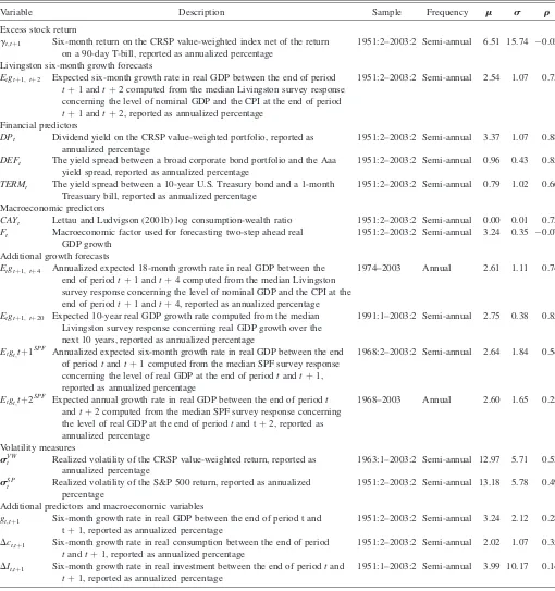
Here, we introduce the data and document some of their properties. Unless noted otherwise, all data are measured biannually. In Table 1 we report the name and a short description of each series as well as its frequency, available sample range, mean, standard deviation, and first order auto-correlation coefficient.
Excess Stock Returns. We construct excess stock returns using the Center for Research and Security Prices (CRSP) value-weighted portfolio and the 90-day U.S. Treasury bill rate, 1952:1–2003:2.
Livingston Six-Month Growth Forecasts. The Livingston survey is widely followed, heavily studied, and generally respected, as surveyed, for example, by Croushore (1997). Moreover, and importantly, it is available over a long sample period, in contrast, for example, to the Survey of Professional Forecasters, which began in 1968. The Livingston survey is biannual, conducted in June and December. Our sample begins in 1952:1, which matches the beginning of the continuously-recorded Livingston survey data, and continues until 2003:2. Note the notation associated with the biannual data: 2001:2, for example, refers to the second half of 2001 (i.e., 7/1/2001 through 12/31/2001).
We construct real gross domestic product (GDP) growth expectations from nominal GDP and consumer price index
‘‘. . . [if] cyclical variation in the market risk premium is present,. . .we would expect to find evidence of it from forecasting regressions of excess returns on macroeconomic variables over business cycle horizons. Yet the most widely investigated predictive variables have not been macroeconomic varia-bles, but financial indicators.’’ (Lettau and Ludvigson 2005b)
266
2009 American Statistical Association Journal of Business & Economic Statistics April 2009, Vol. 27, No. 2 DOI 10.1198/jbes.2009.0025
(CPI) level expectations reported in the Livingston survey, which solicits respondents’ views regarding economic varia-bles in six and 12 months’ time. Unfortunately, the Livingston survey does not ask participants about expectations ofcurrent
GDP or CPI levels, so we cannot use it to construct one-step-ahead forecasts (a step being a six-month interval). We aggregate the Livingston responses into median forecasts, obtaining, for each series and survey date, a median forecast of the series’ level six and 12 months hence, and we take log
differences to obtain an approximate two-step-ahead growth rate forecast, as in Gultekin (1983). The final result is a series of two-step-ahead real GDP growth forecasts, Et gtþl, tþ2 spanning 1952:1–2003:2.
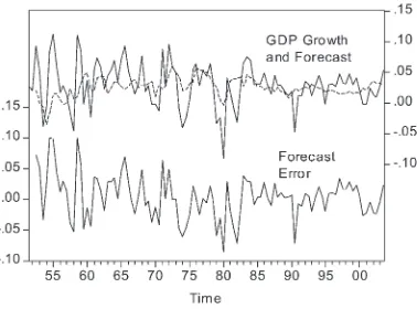
The two-step-ahead real growth rate forecasts constructed from the Livingston data appear well behaved. In Figure 1 we show the actual growth rates, the Livingston forecasts, and the corresponding forecast errors. The forecasts move with the actual growth rates but are smoother, which is a well-known
Table 1. Variable descriptions and descriptive statistics
Variable Description Sample Frequency m s r
Excess stock return
gt,tþ1 Six-month return on the CRSP value-weighted index net of the return on a 90-day T-bill, reported as annualized percentage
1951:2–2003:2 Semi-annual 6.51 15.74 0.02
Livingston six-month growth forecasts
Etgtþ1,tþ2 Expected six-month growth rate in real GDP between the end of period
tþ1 andtþ2 computed from the median Livingston survey response concerning the level of nominal GDP and the CPI at the end of period
tþ1 andtþ2, reported as annualized percentage
1951:2–2003:2 Semi-annual 2.54 1.07 0.73
Financial predictors
DPt Dividend yield on the CRSP value-weighted portfolio, reported as
annualized percentage
1951:2–2003:2 Semi-annual 3.37 1.07 0.88
DEFt The yield spread between a broad corporate bond portfolio and the Aaa
yield spread, reported as annualized percentage
1951:2–2003:2 Semi-annual 0.96 0.43 0.85
TERMt The yield spread between a 10-year U.S. Treasury bond and a 1-month
Treasuary bill, reported as annualized percentage
1951:2–2003:2 Semi-annual 0.79 1.02 0.66
Macroeconomic predictors
CAYt Lettau and Ludvigson (2001b) log consumption-wealth ratio 1951:2–2003:2 Semi-annual 0.00 0.01 0.72
Ft Macroeconomic factor used for forecasting two-step ahead real
GDP growth
1951:2–2003:2 Semi-annual 3.24 0.35 0.07
Additional growth forecasts
Etgtþ1,tþ4 Annualized expected 18-month growth rate in real GDP between the end of periodtþ1 andtþ4 computed from the median Livingston survey response concerning the level of nominal GDP and the CPI at the end of periodtþ1 andtþ4, reported as annualized percentage
1974–2003 Annual 2.61 1.11 0.74
Etgtþ1,tþ20 Expected 10-year real GDP growth rate computed from the median Livingston survey response concerning real GDP growth over the next 10 years, reported as annualized percentage
1991:1–2003:2 Semi-annual 2.75 0.38 0.85
Etgt;tþ1
SPF Annualized expected six-month growth rate in real GDP between the end
of periodtandtþ1 computed from the median SPF survey response concerning the level of real GDP at the end of periodtandtþ1, reported as annualized percentage
1968:2–2003:2 Semi-annual 2.64 1.84 0.54
Etgt;tþ2
SPF
Expected annual growth rate in real GDP between the end of periodt
andtþ2 computed from the median SPF survey response concerning the level of real GDP at the end of periodtand tþ2, reported as annualized percentage
1968–2003 Annual 2.60 1.65 0.25
Volatility measures
sVWt Realized volatility of the CRSP value-weighted return, reported as
annualized percentage
1963:1–2003:2 Semi-annual 12.97 5.71 0.53
sSPt Realized volatility of the S&P 500 return, reported as annualized
percentage
1951:2–2003:2 Semi-annual 13.18 5.78 0.49
Additional predictors and macroeconomic variables
gt,tþ1 Six-month growth rate in real GDP between the end of period t and tþ1, reported as annualized percentage
1951:2–2003:2 Semi-annual 3.24 2.12 0.28
Dct,tþ1 Six-month growth rate in real consumption between the end of period
tandtþ1, reported as annualized percentage
1951:2–2003:2 Semi-annual 2.02 1.07 0.35
DIt,tþ1 Six-month growth rate in real investment between the end of periodtand
tþ1, reported as annualized percentage
1951:1–2003:2 Semi-annual 3.99 10.17 0.14
NOTE: We report the notation and description of each variable in the first and second column. The sample range of each variable is reported in the third column. The frequency of each series is reported in the fourth column. The sample mean, standard deviation, and first-order autocorrelation coefficient of each variable is reported in the fourth, fifth, and sixth column.
property of optimal forecasts of stationary series (e.g., see Diebold 2007). Moreover, the forecast errors appear to have zero mean and display no obvious predictable patterns. The sharp cutoff in the sample autocorrelation function of the forecast errors beyond displacement one, as shown in Figure 2, indicates first-order moving average structure, which is con-sistent with optimality of the two-step-ahead forecasts. The mean Livingston (annualized) real GDP growth rate forecast in Table 1 is 2.54%, which closely accords with historical growth realizations.
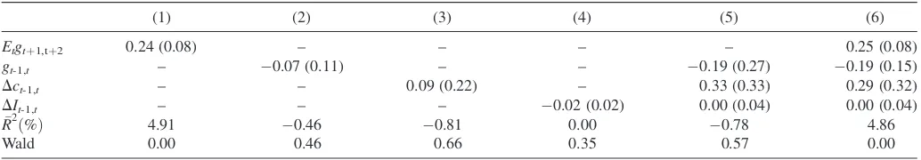
In Table 2, we examine the performance of the Livingston forecasts in more detail by regressing realized real GDP growth, two steps ahead, on the Livingston forecasts as well as lagged real GDP growth, real consumption growth, and real investment growth. The first column of Table 2 indicates that the Livingston growth forecasts are informative about future real GDP growth; the forecasts predict future growth
with at-statistic of 3.0. When compared with the forecasting performance of lagged real GDP, consumption, and investment growth the Livingston forecast stands out. Specifically, in each of the univariate specifications only the Livingston forecast is a significant predictor of future GDP growth. Moreover, when the Livingston forecast is combined with the other predictors the size and significance of the coefficient on the Livingston forecast is unaffected. Accordingly, the Livingston forecast contains important information about future real GDP growth, which is not contained in other macroeconomic variables.
Financial Predictors. We examine several standard and widely studied financial return predictors, the dividend yield,
DPt, calculated for the CRSP value-weighted portfolio, the default premium, DEFt, calculated as the yield difference between a broad corporate bond portfolio and the Aaa yield, and the term premium,TERMt, calculated as the yield differ-ence between a 10-year Treasury bond and a one-month Treasury bill, also 1952:1–2003:2. We also examined Santos and Veronesi’s (2006) ratio of labor income to consumption and Bollerslev and Zhou’s (2006) variance risk premium. Both of those variables, however, were consistently insignificant, so we omit them from the results that follow.
Macroeconomic Predictors. We also examine two mac-roeconomic stock return predictors. The first is Lettau and Ludvigson’s (2001a, b) consumption wealth ratio, CAYt. The second is a simple alternative to the survey expectations of future expected real GDP growth. Specifically, we consider a forecast of future real GDP growth, Ft,based on lagged real GDP growth, consumption growth, and investment growth. We construct the forecast from the estimates in column (5) of Table 2. Each of these macroeconomic predictors spans 1952:1– 2003:2.
Additional Growth Forecasts. The Livingston six-month growth forecast,Etgtþi,tþ2, is our primary measure of expected future business conditions. We do, however, examine the robustness of our findings to other measures of expected future business conditions. We now briefly describe these additional expectations data.
Beginning in 1974, the December Livingston survey asks participants for their expectations of nominal GDP and CPI levels in two years’ time. We use this data in conjunction with the survey expectations for nominal GDP and the CPI levels in six months’ time to construct a measure of expected real GDP growth over the 18-month period beginning in six months’ time,
Etgtþl,tþ4. The data are annual and span the 1974–2003 period. Beginning in 1991, the Livingston survey asks participants for their expectations of real GDP growth over the next 10 years. This long-term growth expectation,Etgt,tþ20, is meas-ured in both the June and December survey and spans the 1991:1–2003:2 period.
The Survey of Professional Forecasters (SPF) is an alter-native survey of expected business conditions. It is a quarterly survey, which we aggregate to biannual for comparability with our other analyses. It is unfortunately available only over a significantly shorter period than the Livingston survey, but it also has some useful features that Livingston does not. Beginning in 1968, the SPF asks participants for their expect-ations for the level of real GDP in the current period and in six
Figure 1. Real GDP growth, Livingston forecast, and Livingston forecast error. Notes: On the right scale we show U.S. biannual real GDP and the corresponding Livingston forecast. On the left scale we show their differences, the forecast error. See text for details.
Figure 2. Sample autocorrelation function two-step ahead real GDP growth forecast errors. Notes: We report the sample autocorrelation function of two-step-ahead Livingston real GDP growth forecast errors, 1952:1–2003:2, along with approximate 95% confidence intervals under the null hypothesis of white noise. The forecasts are made biannually, so the autocorrelation displacement is measured in units of six months. Hence, for example, a displacement of two cor-responds to one year. The Ljung-Box statistic for testing the hypoth-esis of zero autocorrelations at displacements 2–25 is 18.76, which is insignificant at any conventional level. See text for details.
months’ time. Because the SPF asks participants about their expectations for the current level of real GDP (unlike the Livingston survey), we can construct one-step-ahead forecasts for real GDP growth,EtgSPFt;tþ1
;which span 1968:1–2003:2.
Beginning in 1968, the SPF asked participants for their expectations for the level of real GDP in the current period and in 12 months’ time. We use these data to construct a measure of expected real GDP growth over the following 12 months,
EtgSPFt;tþ2
;which spans 1968–2003.
Volatility Variables. We use data on the realized vola-tility of the CRSP value-weighted daily return,sVWt
;tþ1
;which is
available 1963:1–2003:2, as well as data on the realized vol-atility of the S&P 500 daily return,sSPt
;tþ1
; which is available
over the full sample period 1952:1–2003:2.
Additional Predictors and Macroeconomic Varia-bles. We also use data on the growth rate of real GDP,gt,tþl, consumption, Dct,tþl, and investment, DIttþl, from 1952:1– 2003:2 to construct a macroeconomic factor that predicts real GDP growth. We call that factorFt.
3. RELATIONSHIPS AMONG EXPECTED BUSINESS CONDITIONS, FINANCIAL RETURN PREDICTORS,
AND MACROECONOMIC RETURN PREDICTORS
In their classic assessment of the predictability of excess stock returns, Fama and French (1989) found that excess returns are indeed predictable, with most predictive power coming from the dividend yield, the default premium, and the term premium. More precisely, they estimate regressions of the form
Rt;tþh¼b0þb1DPtþb2TERMtþb3DEFtþ
et
;tþh; ð1Þ
and they document a strong relationship in terms of the usualt -statistics, R2 values, and so forth, where Rt,tþh is the excess return on a broad stock portfolio overhperiods, forhranging from one quarter to several years.
The Fama-French research program stresses the role that financial predictors play in predicting stock returns. More recently, researchers have found evidence that macroeconomic variables also may play a role in predicting stock returns. Lettau and Ludvigson (2001b), for example, found that the ratio of consumption to wealth,CAYt, predicts stock returns.
The key open question iswhyfinancial and macroeconomic variables should predict excess returns. In the case of the financial predictors, Fama and French (1989) suggested that the predictive power may derive from their correlation with
expected business (i.e., macroeconomic) conditions. In the case of the macroeconomic predictors, it is also possible that at least part of their predictive power stems from their information content about future real activity.
Notoriously little direct evidence exists, however, as to whether these financial and macroeconomic variables actually
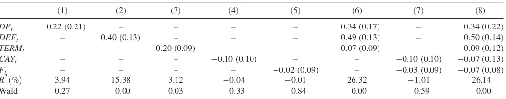
are linked to expected business conditions. In this section we provide precisely such direct evidence, examining the extent to which the Livingston real growth expectations are linked to the standard financial and macroeconomic predictors, both pair-wise and jointly. We estimate regressions of Livingston expected business conditions Etgtþl,tþ2on the financial pre-dictors (DPt,DEFt,TERMt) and onCAYtas well as our mac-roeconomic databased measure of expected future real GDP growth,Ft.In Table 3 we show results from both simple and multiple regressions.
First, consider the relationship between the financial pre-dictors and the Livingston forecasts. The simple regressions reveal some links between the financial variables and expected business conditions, although the strength and statistical sig-nificance vary across variables and specifications. First, the dividend yield is negatively, though insignificantly, related to expected business conditions. This accords with the dividend discount model with a constant expected return, which predicts that the dividend yield should fall when necessary to offset higher expected growth in dividends. Second, the term pre-mium is positively related to expected business conditions. This accords with the basic notion that the yield curve slope is a leading indicator, with inverted yield curves indicating a likely future recession, due, for example, to tightening of monetary policy, which increases short rates. Finally, the default pre-mium appears positively associated with expected business conditions. This seemingly anomalous result may be due to the short horizons associated with the Livingston forecasts; that is, notwithstanding the positive correlation between default pre-mia and expected business conditions at short horizons, default premia may be negatively correlated with expected business conditions at longer horizons of, say, two or three years.
The multiple regressions in Table 3 provide a summary distillation of the links between expected real business con-ditions and the financial variables, taken jointly as a set. The results show that expected business conditions are indeed systematically linked to the financial variables, with R2’s of roughly 25%. This is particularly noteworthy given the short horizons of the Livingston expectations, because the dividend yield and term premium variables—in addition to the default
Table 2. The predictive content of the Livingston six-month growth forecasts
(1) (2) (3) (4) (5) (6)
Wald 0.00 0.46 0.66 0.35 0.57 0.00
NOTE: We report OLS estimates of regressions of real GDP growth,gtþl, onto the Livingston six-month growth forecasts and several other macro predictors, 1952:1–2003:2, with
Newey-West robust standard errors in parentheses. We also report the adjustedR2,R2, as well as thep-value of the Wald test that none of the included variables forecast future real GDP growth in the final two rows of the table.
premium as already discussed—are often thought to have maximal predictive value at much longer horizons.
Now consider the relationship between the macroeconomic variables and the Livingston forecasts. The simple regressions show only a weak association between the Livingston forecasts and each of the macroeconomic variables. In each case the estimated relationship is weak, with a negative adjusted R2. The multiple regression results echo the simple regression results. Taken together, the three macroeconomic variables only account for a small portion of the variation in the Liv-ingston forecasts. In this sense, the LivLiv-ingston forecasts contain considerable information regarding expectations about future business conditions over and above any that may be contained in the macroeconomic variables. Hence, the Livingston fore-casts provide an excellent opportunity to examine the role that expectations about future real activity play in predicting future stock returns.
In summary, the results of this section help us to understand why the standard financial variables ‘‘work’’ in predictive regressions for excess stock returns: They are correlated with expected business conditions, as conjectured by Fama and French (1989). Crucially, however, the correlation is far from perfect (R20.3). That is, the financial variables, even when taken jointly as a set, provide only highly noisy proxies of expected business conditions. This suggests that, to the ex-tent that expected excess returns are driven by expected busi-ness conditions, superior return predictions may be produced via a direct measure of expected business conditions. We now provide precisely such a direct assessment of the effects of expected business conditions on expected excess stock returns.
4. EXPECTED BUSINESS CONDITIONS AND EXPECTED EXCESS RETURNS
Thus far we have established that the standard financial predictors are indeed correlated with expected business con-ditions. Now we go the full mile, asking whether expected business conditions do indeed predict excess returns. We pro-ceed in three steps. First, in Section 4.1 we focus on the pre-dictive ability of the Livingston six-month growth forecasts, controlling for a variety of other predictors. Second, in Section 4.2 we retain focus on the Livingston six-month forecasts, but we assess robustness to the return horizon, different sample periods, and different timing conventions. Finally, in Section
4.3 we explore other (non-Livingston) measures of expected business conditions.
4.1 Main Results: Livingston Six-Month Growth Forecasts
We now consider the central question of whether and how expected business conditions are linked to expected excess returns. We regress excess stock returns on the Livingston six-month growth forecasts, Et gtþ1, tþ2, as well as additional financial and macroeconomic predictors,
Rtþ1;tþ2¼aþbEtgtþ1;tþ2þg
9Xtþetþ1
;tþ2; ð2Þ
where the timing of the excess returnRtþ1,tþ2matches that of expected business conditionsEtgtþ1,tþ2, and where we stand-ardize all predictors to have zero mean and unit variance to facilitate comparison of coefficient magnitudes.
Note that the predictive regression (2) involves a two-step-ahead forecast rather than the one-step-two-step-ahead forecast com-monly employed in the literature. We focus on two-step-ahead forecasts for two reasons. First, there is some uncertainty as to the precise time when the growth forecasts are made, because they are constructed from surveys, and some forecasts may in fact be made after the end of June or December, resulting in an overlap in the information sets from whichEtgtþ1,tþ2andRt,tþ1 are derived. Focusing on forecasts ofRtþ1,tþ2rather thanRt,tþ1 guards against this possibility. Second, and most importantly and obviously, pairingRtþ1,tþ2withEtgtþ1,tþ2matches the timing of the excess return to the horizon of the growth forecast.
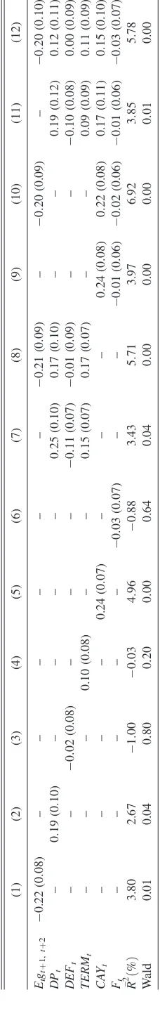
We show the results in Table 4. First, consider the simple regressions in columns (1)–(6), in which we include the various predictors one at a time, and consider in particular the results for the Livingston six-month growth forecasts. The point estimate indicates an economically important negative rela-tionship between expected excess returns and expected busi-ness conditions, with a one standard deviation decrease inEt
gtþ1,tþ2producing roughly a 0.2 standard deviation increase in expected excess returns. The relationship is highly statistically significant at any conventional level, and the adjusted R2 is quite high (for the return-prediction literature) at 3.80%.
The simple regression results for the standard financial pre-dictors,DPt,TERMt, andDEFt, reported in columns (2)–(4), are comparatively lackluster. The coefficient point estimates for the financial predictors are all smaller than that for Et gtþ1,tþ2;
Table 3. Regressions of Livingston six-month growth forecasts on financial and Macro predictors
(1) (2) (3) (4) (5) (6) (7) (8)
Wald 0.27 0.00 0.03 0.33 0.84 0.00 0.59 0.00
NOTE: We report OLS estimates of regressions of real GDP growth expectations,Etgtþl,tþ2, on several predictors, 1952:1–2003:2, with Newey-West robust standard errors in
parentheses. We also report the adjustedR2,R2, as well as thep-value of the Wald test that none of the included variables are related to the Livingston forecasts in the final two rows of the table. We standardized all variables. See text for details.
indeed, those forTERMt, andDEFtare less than half that ofEt
gtþ1,tþ2. Similarly, the significance levels for the conventional predictors are weaker than that forEtgtþ1,tþ2, andTERMtand
DEFt are statistically insignificant at any conventional level. Finally, the adjustedR2values for the conventional predictors are all smaller than that for Et gtþ1,tþ2, and those forTERMtand
DEFtare negligible.
The simple regression results for the macroeconomic pre-dictors,CAYtandFt, reported in columns (5)–(6), show thatCAYt is a strong predictor of excess returns, whereasFtis not. In the case of the macroeconomic databased forecast of future growth,
Ft,the point estimate is negative, which supports the notion that better expected future business conditions forecast lower excess returns though the point estimate is small and insignificant.
Now consider the multiple regression results reported in columns (7)–(12) of Table 4. Columns (7) and (8) show the effect of adding the Livingston six-month forecast to a regression of excess stock returns on financial predictors. The point estimates in column (7) reveal that the dividend yield is the strongest predictor among the financial predictors. Adding the Livingston forecast, in column (8), reduces both the size of the dividend yield coefficient estimate and its t-statistic by roughly one-third, while simultaneously raising the adjustedR2
by more than 60%. Columns (9) and (10) show the effect of adding the Livingston forecast to a regression of excess stock returns on macroeconomic predictors. The Livingston survey continues to have a sizable and significant effect on future excess returns, nearly doubling the adjustedR2of the forecast based solely on macroeconomic predictors. Columns (11) and (12) show the effect of adding the Livingston forecast to a specification that includes both financial and macroeconomic predictors. Even after controlling for both sets of predictors, the Livingston forecast has a large and significant negative effect on future returns, resulting in roughly a 50% increase in the adjustedR2of the forecast.
All told, the results in Table 4 clearly point to expected business conditions as a key determinant of expected excess returns. Across each specification, we find that the Livingston forecast is negatively related to future excess returns, and this effect is always significant at standard significance levels. Moreover, the quantitative impact of expected future business conditions is large. Only CAYt is estimated to have a larger effect on excess stock returns and including the Livingston forecast always improves the adjusted R2 of the multiple regression specifications.
4.2 Variations I: Alternative Return Horizons, SubSample Analysis, and Timing
The results thus far indicate that expected business con-ditions play a key role in forecasting excess returns. Relative to other predictors employed in the literature, the forecasting power of the Livingston six-month growth forecasts is large and significant. In this subsection we consider three important extensions, assessing whether the results are stable across alternative return horizons, subsamples, and alternative return timing conventions.
Return Horizon. The results thus far provide clear evi-dence that expected business conditions help to forecast excess
T
returns at a six-month horizon. Now, we examine the value of expected business conditions in forecasting excess returns at various longer horizons. We measure the long-horizon regres-sion coefficients on the Livingston six-month growth forecast,
Et gtþ1,tþ2, using Hodrick’s (1992) unified vector autore-gression (VAR) methodology, which produces predictive regression coefficients and R2’s at all horizons from a single underlying VAR.
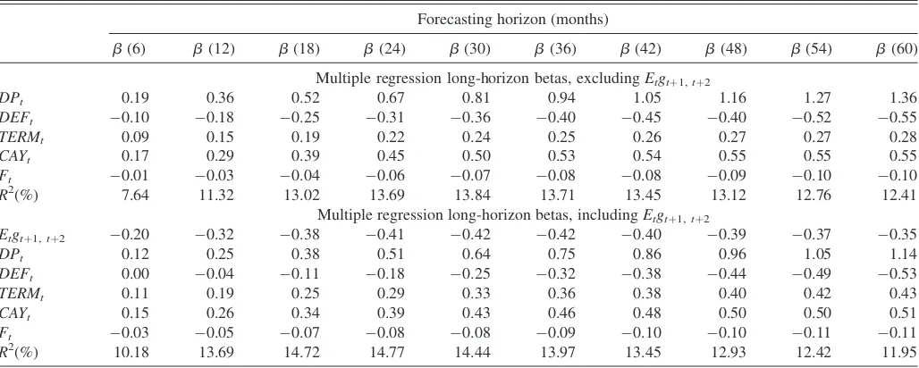
In Table 5 we report long-horizon regression statistics for horizons ranging from six to 60 months. As before, we stand-ardize each predictor, so that we can compare the imputed long-horizon regression coefficients across predictors. In the top and bottom panels of Table 5, we present long-horizon multiple regression statistics implied by the Hodrick VAR system, excluding and including expected business conditions, respectively. Each panel contains multiple regression coef-ficients for each forecasting horizon and the impliedR2.
The patterns in the multiple regression coefficients indicate that the effect of including expected business conditions dis-sipates as the forecasting horizon lengthens. This is most evi-dent when comparing the effect of the dividend yield to that of expected business conditions. Inclusion of expected business conditions reduces the dividend yield coefficient by roughly 40% at the six month horizon, whereas it reduces it by only 15% at the 60 month horizon. A similar pattern arises for the long-horizonR2’s. At the six month horizon, adding expected business conditions to the set of predictors increases theR2by roughly 33%. At horizons beyond 24 months, including expected business conditions produces only negligible changes in return predictability.
The general pattern in coefficients and predictability at horizons beyond six months indicates that expected business conditions are most useful for predicting excess returns over the six to 24month horizon. This finding is appealing. It is consistent with both the short- to medium-term nature of the Livingston forecasts, and with the possibility that other
pre-dictors contain information, not contained in the Livingston forecasts, of relevance for forecasting longer-term excess returns. Quite naturally, then, the information content of the Livingston forecasts appears most relevant over the horizons to which they are tailored. Recently, the Livingston survey has added forecasts of longer-run growth (18 months and 10 years ahead), which we subsequently examine.
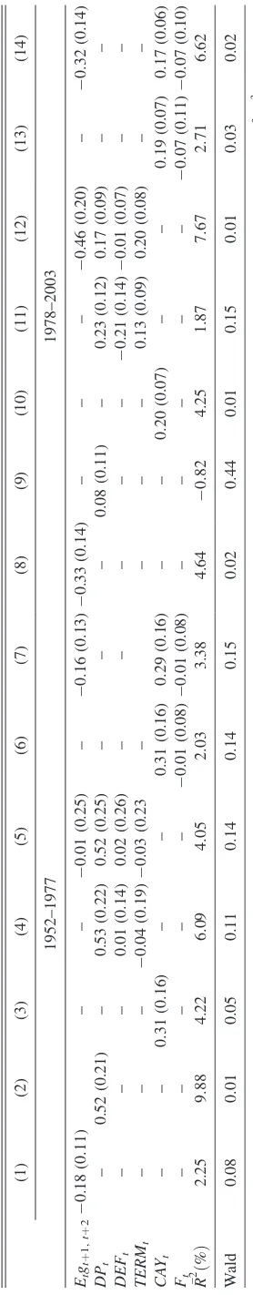
Subsamples. Although the full sample results presented in Table 4 indicate that expected business conditions have a strong and negative effect on future excess returns, it is worth con-sidering whether this finding is robust across subsamples. Hence, we break the full sample into two equal periods: 1952:1–1977:2 and 1978:1–2003:2. In Table 6, we report estimates of the most important specifications from Table 4 over the two subsamples.
Columns (1)–(3) and (8)–(10) show estimates of the simple regressions over the two subsamples for the three most important predictors of excess returns identified in Table 4,
Et gtþ1,tþ2, DPt, and CAYt. The predictive contents of the Livingston forecast, Et gtþ1,tþ2, and the consumption-wealth ratio, CAYt, are relatively stable over the two subsamples. In each case, the point estimates vary within a relatively narrow range and exhibit similar degrees of statistical significance across both subsamples. In contrast, the predictive content of the dividend yield, DPt, varies considerably across the two subsamples. In the early subsample the dividend yield strongly predicts future excess returns, both in terms of its estimated effect and statistical significance. In the late subsample the point estimate is considerably smaller (0.08 versus 0.52) and insignificant. Moreover, the adjusted R2 over the late sub-sample is actually negative.
Columns (4)–(5) and (11)–(12) compare the effect of adding the Livingston six-month growth forecast to a multiple regression that only employs financial predictors. In both subsamples, adding the Livingston forecast to the financial predictors results in a negative point estimate, although the
Table 5. Long-horizon regressions of excess stock returns on six-month growth forecasts, financial predictor, and Macro predictors
Forecasting horizon (months)
b(6) b(12) b(18) b(24) b(30) b(36) b(42) b(48) b(54) b(60)
Multiple regression long-horizon betas, excludingEtgtþ1,tþ2
DPt 0.19 0.36 0.52 0.67 0.81 0.94 1.05 1.16 1.27 1.36
DEFt 0.10 0.18 0.25 0.31 0.36 0.40 0.45 0.40 0.52 0.55
TERMt 0.09 0.15 0.19 0.22 0.24 0.25 0.26 0.27 0.27 0.28
CAYt 0.17 0.29 0.39 0.45 0.50 0.53 0.54 0.55 0.55 0.55
Ft 0.01 0.03 0.04 0.06 0.07 0.08 0.08 0.09 0.10 0.10
R2(%) 7.64 11.32 13.02 13.69 13.84 13.71 13.45 13.12 12.76 12.41
Multiple regression long-horizon betas, includingEtgtþ1,tþ2
Etgtþ1,tþ2 0.20 0.32 0.38 0.41 0.42 0.42 0.40 0.39 0.37 0.35
DPt 0.12 0.25 0.38 0.51 0.64 0.75 0.86 0.96 1.05 1.14
DEFt 0.00 0.04 0.11 0.18 0.25 0.32 0.38 0.44 0.49 0.53
TERMt 0.11 0.19 0.25 0.29 0.33 0.36 0.38 0.40 0.42 0.43
CAYt 0.15 0.26 0.34 0.39 0.43 0.46 0.48 0.50 0.50 0.51
Ft 0.03 0.05 0.07 0.08 0.08 0.09 0.10 0.10 0.11 0.11
R2(%) 10.18 13.69 14.72 14.77 14.44 13.97 13.45 12.93 12.42 11.95
NOTE: We report long-horizon regression coefficients andR2values for horizons ranging from six to 60 months, 1952:1–2003:2. In the top panel, we report multiple regression
coefficients andR2values for a specification that excludes Livingston six-month growth forecasts as a predictor. In the bottom panel we report coefficients andR2values for a
specification that includes the Livingston forecast as a predictor. We standardized all predictors. See text for details.
point estimate in the early subsample is smaller in magnitude and statistically insignificant. In the early subsample the large and significant effect of the dividend yield tends to crowd out the Livingston forecast. Columns (6)–(7) and (13)–(14) com-pare the effect of adding the Livingston forecast to a multiple regression that only employs macroeconomic predictors. Across both subsamples the Livingston forecast has a sizeable negative effect on future excess returns that is similar to the simple regression point estimate from each subsample.
All told, the results of the subsample analysis in Table 6 indicate that the effect of the Livingston six-month forecasts on future excess returns is relatively stable. In the case of the simple regressions, the point estimates are negative, of similar magnitude (0.2 and 0.3), and of similar statistical sig-nificance across both periods. In the case of the multiple regressions, higher growth forecasts are associated with lower future excess returns in every specification. Although the div-idend yield crowds out much of the effect of the Livingston forecasts in the early subsample, this should be tempered by the fact that the effect of the dividend yield is unstable across the different subsamples.
Return Timing. Thus far we have presented evidence that expected business conditions forecast excess returns based on variants of Equation (2),Rtþ1,tþ2¼b0þb1Etgtþ1,tþ2þg9Xt
þetþ1,tþ2, in which we regress two-step-ahead excess returns on the Livingston six-month forecasts and other predictors. Although we have argued that this is the most appropriate timing convention given the timing of the survey and the horizon of the growth forecasts, it is worthwhile to examine whether the predictive content of the Livingston forecasts is sensitive to this timing convention. We do this by estimating the following regression,
Rt;tþ1¼aþbEtgtþ1;tþ2þg
9Xtþetþ1
;tþ2; ð3Þ
which uses the one-step-ahead excess return,Rt,tþ1, rather than the two-step-ahead excess return, Rtþ1,tþ2, as the dependent variable. We report the results in Table 7. The specifications that we examine in Table 7 are identical to those in Table 4.
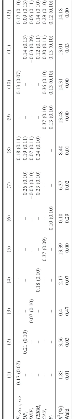
The point estimate on the Livingston forecasts in the simple regression, reported in column (1), is 0.17, which is sig-nificant at the 1% level though reduced somewhat relative to the result in Table 4 (0.22). Looking across each of the simple regression specifications in columns (1)–(6) of Table 7 shows that the results are similar to those reported in Table 4. In particular, both DPt and CAYt are identified as significant predictors of excess returns in the simple regressions, with point estimates that are similar in size and significance to those reported in Table 4. One important difference between these results and those reported in Table 4 is that, over the one-step-ahead horizon, the forecasting power ofCAYtdominates that of the Livingston forecasts and all of the other predictors that we examine. Over this horizon and this sample period the fore-casting power of CAYtis quite remarkable, whereas the fore-casting power of the Livingston forecasts is more in line with that reported earlier.
All told, the simple and multiple regression results reported in Table 7 indicate that the effect of the Livingston forecasts on future excess returns is robust to differences in the precise
T
timing of excess returns. In particular, across all specifications we find that the point estimate is negative, similar in magnitude to that reported in Table 4, and statistically significant at the 10% level or better in three out of four cases. Moreover, in every case, adding the Livingston six-month forecast improves the adjusted R2 of the regression, further suggesting that expected business conditions are an important determinant of excess stock returns.
4.3 Variations II: Additional Measures of Expected Business Conditions
The six-month Livingston growth forecast,Etgtþ1,tþ2, is our primary measure of expected business conditions due to its long sample period, 1952:1–2003:2, and biannual frequency. These survey forecasts, however, are not the only available measures of expected real GDP growth. In this section we examine the robustness of our results to additional measures of expected business conditions. Specifically, we use two addi-tional measures of expected future real GDP growth from the Livingston survey as well as two measures of expected future real GDP growth from the Survey of Professional Forecasters (SPF). Each of these additional measures is available over a different and shorter sample and in some cases at a lower fre-quency than the Livingston six-month growth forecasts. As a result, the statistical precision of the results that follow is naturally weaker than that of the Livingston six-month growth forecasts. Also, because additional forecasts all have differing sample ranges and frequencies, the precise timing and fre-quency of the following regressions depends on the specific forecast and control variables employed.
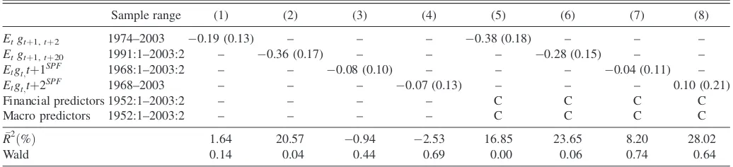
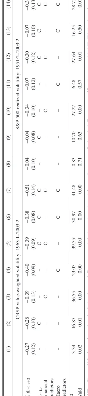
In Table 8 we examine the relationship between excess stock returns and two additional real GDP growth forecasts from the Livingston survey as well as two real GDP growth forecasts from the SPF. We run each regression in Table 8 using a set of nonoverlapping observations as in Tables 4–7. We also specify each regression to make the horizon of the excess return close to the horizon of the corresponding growth forecast wherever possible. Finally, to avoid unnecessary distraction, we show only point estimates and standard errors for the estimated coefficients on the additional growth forecasts, using a ‘‘C’’ to denote that a predictor has been controlled for in the regression. The first additional growth forecast that we examine in Table 8 is the Livingston survey’s annual (December) forecast of growth over the 18-month period beginning in 6 months’ time,
Etgtþ1,tþ4. This forecast provides a slightly longer term view of the macroeconomy than the six-month forecast,Etgtþ1,tþ2, but it is only available at the annual frequency, and only since 1974. Given its annual frequency, we regress annual excess returns on the lagged value of the forecast, Rt,tþ2 ¼ a þ bEt(gtþ1,tþ4)þg9Xtþet,tþ2. We consider two specifications, reported in columns (1) and (5). In a simple regression of excess returns on this forecast we find a negative relationship between the forecast and future excess returns that is similar in size to the estimate reported for the Livingston six-month growth forecast in Tables 4, 6, and 7. The point estimate,
0.19, however, is statistically insignificant at standard levels. When we control for the financial and macroeconomic pre-dictors in column (5), the point estimate is still negative, and
T
its magnitude increases to0.38 and is significant at the 5% level.
Next, we consider the Livingston forecast of real GDP growth over the next 10 years following each survey (June and December), Et gt,tþ20. This forecast provides for a long-term view of the macroeconomy and is biannual but is only available since 1991:1. In this case we simply regress our biannual excess returns on the lagged value of the forecast,Rt,tþ1¼aþ bEt(gt,tþ20)þg9Xt þet,tþ2, because matching the horizon of the excess return with that of the forecasts is impractical over the available sample. The results, reported in columns (2) and (6), are also supportive of a negative relationship between expected business conditions and excess returns. In each specification, the point estimate is negative, large in magni-tude, and statistically significant.
We now consider the growth forecasts from the SPF. The first forecast that we examine is the SPF forecast of real GDP growth over the six-month period immediately following the survey,EtgSPFt;tþ1
;which is closest in spirit to the Livingston
six-month forecasts. The main drawback to the SPF forecast is its short sample period, 1968:1–2003:2, relative to the Livingston six-month forecasts. In the case ofEtgSPFt;tþ1
;we regress the
one-step-ahead growth forecast on one-step ahead biannual excess returns, Rt;tþ1¼aþbEtg
SPF
t;tþ1þg‘Xtþ
et
;tþ1: We report the
results in columns (3) and (7). In each specification we find a negative though insignificant relationship. We also consider the SPF forecast of annual real GDP growth as well,EtgPSPEt;tþ2:In
this case we regress annual excess returns on the lagged SPF forecast, Rt;tþ2¼aþbEtg
SPE
t;tþ2þg‘Xtþ
et
;tþ2: We report the
results in columns (4) and (8). In both cases we find that the estimates are not statistically significant at standard levels.
Looking across the range of point estimates presented in Table 8 indicates that additional measures of expected future business conditions are also negatively related to future excess returns. Although the size and significance of the point esti-mates vary, the overall pattern is clear. In 7 of 8 specifications we find a negative relationship between survey-based forecasts of future business conditions and excess returns. Although the general pattern in the results is clear, it is important to note that the statistical significance of the results reported in Table 8 are weaker than those reported for the six-month Livingston forecasts in Tables 4, 6, and 8. Two points regarding the stat-istical significance of the results are worth considering. First,
the additional forecasts that we examine in Table 7 are avail-able only over a shorter sample period than that of the Liv-ingston six-month forecasts. Second, the measures of statistical significance that we report are marginal rather than joint and thus do not account for the breadth and consistency of the results across the entire set of additional forecasts.
5. DISCUSSION
We have documented a robust negative correlation between expected excess returns and expected business conditions, so that, for example, low expected future growth is associated with high current expected excess stock returns. Here we address an important issue: Why thenegativerelationship? Our answer is 2-fold.
First, the high persistence of real activity over the business cycle should contribute to a negative relationship. In particular, business cycle regimes (especially expansions) typically last for much longer than six to 12 months, so the rational forecast is ‘‘good times now, likely good times in the future,’’ and conversely. Hamilton’s (1989) classic Markov-switching analysis, for example, produces one-step (quarterly) ‘‘staying probabilities’’ of p1
11 ¼0:9 for expansions andp
1
00¼0:75 for
contractions. Iterating forward we obtain two-quarter staying probabilities ofp2
11¼0:84 for expansions andp
2
00¼0:59 for
contractions. Hence, over the horizons of one or two quarters of most relevance for our analysis, current conditions are more likely to persistthan to reverse. The Livingston expectations rationally reflect that fact, rendering them positively rather than negatively correlated with current conditions, and hence neg-atively related to expected excess returns. This contrasts with—but in no way contradicts—the fact emphasized in the recent finance literature that over very longhorizons current conditions are likely to mean-revert.
Second, expected business conditions may forecast future volatility and hence may be linked to perceived systematic risk and expected excess returns. The claim that business conditions are linked to stock market volatility is certainly not new. In particular, as persuasively documented in an extensive study by Schwert (1989) and echoed in subsequent work by Hamilton and Lin (1996) using very different and complementary methods, stock market risk increases in recessions. Indeed, in our view real activity is the only important and robust covariate
Table 8. Regressions of excess stock returns on alternative growth forecasts, financial predictors, and Macro predictors
Sample range (1) (2) (3) (4) (5) (6) (7) (8)
Financial predictors 1952:1–2003:2 – – – – C C C C
Macro predictors 1952:1–2003:2 – – – – C C C C
R2ð%Þ 1.64 20.57 0.94 2.53 16.85 23.65 8.20 28.02
Wald 0.14 0.04 0.44 0.69 0.00 0.06 0.74 0.64
NOTE: We report OLS estimates of regressions of excess returns on alternative growth forecasts, a set of financial predictors,DPt,DEFt,TERMt, and a set of macro predictors,CAYt,Ft,
with Newey-West standard errors in parentheses. We use a ‘‘C’’ to denote that a set of variables has been controlled for in the regression. The sample range and frequency of each variable is reported in the second column. The range and frequency of each regression is determined by the shortest sample and lowest frequency of all the included variables. We report the adjustedR2,R2,aswell as thep-value of the Wald test that the corresponding growth forecast does not forecast future excess returns in the final two rows of the table. We standardized all variables. See text for details.
of stock market volatility thus far identified, notwithstanding the many investigations.
In Table 9 we examine the link between expected business conditions and realized stock market volatility. We use two data sources to compute realized biannual stock return volatility. The first is the daily CRSP value-weighted index, which is available since 1963, resulting in a sample from 1963:1 through 2003:2. The second is the daily S&P 500 index, which is available since 1951, resulting in a sample from 1951:2 through 2003:2. Then, we regress realized volatility, stþl,tþ2, on expected business conditions,Etgtþl,tþ2, and the other predictors considered earlier as well as a lag of realized volatility,st1,t. As in Table 8, we show only the point estimates and standard errors on expected business conditions to avoid distraction, using ‘‘C’’ to denote that a predictor has been controlled for.
Consider first the regression results for CRSP-based realized volatility in columns (1)–(7). The results indicate that expected business conditions have highly statistically significant pre-dictive ability for volatility. The estimated relationship between expected business conditions and future volatility agrees with the findings of previous research: Low growth expectations forecast high stock return volatility. Moreover, even after controlling for lagged volatility as well as other financial and macroeconomic predictors, expected business conditions emerge as a highly significant predictor of volatility, with a t-statistic in excess of 2.0 across each of the seven specifications. As in the univariate case, low growth expect-ations presage high future volatility.
Now consider the results for S&P-based realized volatility in columns (8)–(14) of Table 9. The sign of the univariate coef-ficient estimate matches that of the CRSP-based estimate in column (1), although the magnitude of the univariate estimate is smaller for the longer S&P-based sample. The multiple regres-sion results, however, are more uniform across the two samples. In particular, the estimated coefficient for expected business conditions changes only slightly from0.51 in the top CRSP-based panel to0.32 in the S&P-based panel once we control for lagged volatility as well as the financial and macroeconomic predictors, and the t-statistic exceeds 2.5 in both cases. Accordingly, both the CRSP and S&P based volatility measures indicate a negative and statistically significant relationship between expected future business conditions and stock market volatility.
It is worth asking whether the full-sample relationship between expected business conditions and stock market vola-tility documented in Table 9 is robust to subsample analysis. In Table 10 we report selected specifications from Table 9 over the 1952–1977 subsamples (columns 1–6) and the 1978–2003 subsamples (columns 7–12). We report results for both the CRSP and S&P 500 volatility measures.
The early subsample results indicate a negative relationship between expected future business conditions and future stock market volatility in 4 of 6 specifications. The results in the case of the CRSP volatility measure are stronger than for the S&P 500 volatility results. In particular, although sets of point estimates are typically insignificant, the size of the effect of expected future business conditions stock market volatility is typically an order of magnitude larger in the CRSP volatility data than in the S&P 500 data.
T
The late subsample results also indicate that expectations of better economic performance forecast lower stock return vol-atility. Unlike the early subsample, however, both the estimated size of the relationship and the degree of statistical significance are similar across both the CRSP and S&P 500 volatility measures.
All told, there is substantial evidence that expected business conditions have robust predictive ability for volatility. Although the degree of statistical significance is reduced in each of the subsamples, the sign and size of the relationship is largely stable.
6. CONCLUDING REMARKS
Our key result, of course, is that expected business con-ditions are a robust predictor of excess returns. An interesting secondary result is that the Lettau-Ludvigson (2001a, b) gen-eralized consumption/wealth ratio (CAY) is also a robust pre-dictor, in contrast to other predictors that feature prominently in the literature but often ‘‘drop out’’ once expected business conditions and CAY are included. Presumably the varia-tion in expected excess returns is ultimately driven by time-varying expected risk and/or time-time-varying risk aversion. Hence, the question naturally arises as to whether and how expected business conditions and CAY are linked to equity market risk and risk aversion.
We believe that the Livingston business conditions expect-ations likely capture time-varying risk, as we discussed in detail in Section 5. But what of the Lettau-Ludvigson generalized consumption/wealth ratio, CAY? We believe that
CAYlikely captures time-varying riskaversion,via the follow-ing logical chain:
(1) Theoretically, time-variation in expected excess returns is ultimately driven by varying expected risk, time-varying risk aversion, or both;
(2) Empirically, time-variation in expected excess returns is driven by two key predictors, expected business conditions andCAY;
(3) Expected business conditions are linked to risk; (4) Expected business conditions andCAYare largely unre-lated;
(5) Hence, by elimination, CAY must be linked to risk aversion.
Our assertion that CAYcaptures time-varying risk aversion matches that of Lettau and Ludvigson (2001b) and provides a largely independent confirmation of their work, insofar as we arrive at the insight via a very different route. Note, however, that we do not assert that movements in CAYare exclusively
driven by movements in risk aversion. In particular, our vola-tility forecasting results indicate that movements in CAYare also related to movements in risk.
Interestingly, Lettau and Ludvigson (2002, 2005a) docu-mented that CAY forecasts future investment and cash flows (dividends and earnings). Their findings, however, indicate that the forecasting power of CAY for those variables is con-centrated at relatively long horizons, in contrast to the short/ medium horizons associated with our expected business conditions variable. Accordingly, we conjecture that CAY
T
measures both risk aversion and a risk component unrelated to the risk component forecast by the Livingston expectations.
Both our results and our interpretation are very much in agreement with an emerging empirical view that expected excess returns are counter-cyclical—not only for stocks, as in Lettau and Ludvigson (2001b), but also for bonds, as in Cochrane and Piazzesi (2005) and Ludvigson and Ng (2007). Interestingly, part of the literature emphasizes higher risk in recessions, as in Constantinides and Duffie (1996), and another part emphasizes higher risk aversion in recessions, as in Campbell and Cochrane (1999). Our results unify those two literatures, suggesting that the cyclicality ofbothrisk and risk aversion contributes to the counter-cyclicality of expected excess returns: Growth expectations are procyclical and have a robust negative impact on expected excess returns, andCAY is
countercyclical and simultaneously has a robust positive impact.
ACKNOWLEDGMENTS
The ideas and opinions expressed are those of the authors and should not be interpreted as reflecting the views of the Board of Governors of the Federal Reserve System nor its staff. For invaluable guidance, we thank the editor, associate editor, and three referees. For support, we thank the Humboldt Foundation, the Guggenheim Foundation, the National Science Foundation, and the Wharton Financial Institutions Center. For helpful comments, we thank seminar participants at the Board of Governors of the Federal Reserve System and the Swiss National Bank (Study Center Gerzensee), as well as Andrew Ang, Ravi Bansal, Hui Guo, Martin Lettau, Sydney Ludvigson, Josh Rosenberg, Steve Sharpe, Jessica Wachter, and Kamil Yilmaz. None of those thanked, however, are responsible for the outcome.
[Received August 2006. Revised December 2008.]
REFERENCES
Barro, R. J. (1990), ‘‘The Stock Market and Investment,’’Review of Financial Studies, 3, 115–131.
Bollerslev, T., and Zhou, H. (2006), ‘‘Expected Stock Returns and Variance
Risk Premia,’’Finance and Economics Discussion Series,2007-11,
Wash-ington, DC: Board of Governors of the Federal Reserve System.
Campbell, J. Y. (1991), ‘‘A Variance Decomposition for Stock Returns,’’The
Economic Journal, 101, 157–179.
Campbell, J. Y., and Cochrane, J. H. (1999), ‘‘By Force of Habit: A
Con-sumption-Based Explanation of Aggregate Stock Market Behavior,’’The
Journal of Political Economy, 107, 205–251.
Campbell, J. Y., and Shiller, R. J. (1988), ‘‘The Dividend-Price Ratio and Expectations of Future Dividends and Discount Factors,’’Review of Finan-cial Studies, 1, 195–227.
Chen, N.-F., Roll, R., and And Ross, S. A. (1986), ‘‘Economic Forces and the Stock Market,’’Journal of Business, 56, 383–403.
Cochrane, J. M., and Piazzesi, M. (2005), ‘‘Bond Risk Premia,’’The American Economic Review, 95, 138–160.
Constantinides, G. M., and Duffie, D. (1996), ‘‘Asset Pricing with
Heteroge-neous Consumers,’’The Journal of Political Economy, 104, 219–240.
Croushore, D. (1997), ‘‘The Livingston Survey: Still Useful After All these Years,’’ Business Review (Federal Reserve Bank of Philadelphia), (March), 15–27. Diebold, F. X. (2007),Elements of Forecasting(4th ed.), Cincinnati:
South-Western.
Fama, E., and French, K. (1988), ‘‘Dividend Yields and Expected Stock Returns,’’Journal of Financial Economics, 19, 3–29.
Fama, E., and French, K. (1989), ‘‘Business Conditions and Expected Returns
on Stocks and Bonds,’’Journal of Financial Economics, 25, 23–49.
Fama, E., and French, K. (1990), ‘‘Stock Returns, Expected Returns, and Real Activity,’’The Journal of Finance, 45, 1089–1108.
Ferson, W. E., and Harvey, C. R. (1991), ‘‘The Variation of Economic Risk
Premiums,’’The Journal of Political Economy, 99, 1393–1413.
Gultekin, N. B. (1983), ‘‘Stock Market Returns and Inflation Forecasts,’’The Journal of Finance, 38, 663–673.
Hamilton, J. D. (1989), ‘‘A New Approach to the Economic Analysis of Non-stationary Time Series and the Business Cycle,’’Econometrica, 57, 357–384. Hamilton, J. D., and Lin, G. (1996), ‘‘Stock Market Volatility and the Business
Cycle,’’Journal of Applied Econometrics, 11, 573–593.
Hodrick, R. (1992), ‘‘Dividend Yields and Expected Stock Returns: Alternative Procedures for Inference and Measurement,’’Review of Financial Studies, 5, 357–386.
Lettau, M., and Ludvigson, S. (2001a), ‘‘Resurrecting the Consumption
CAPM: A Cross-Sectional Test When Risk Premia Are Time-Varying,’’The
Journal of Political Economy, 109, 1238–1287.
Lettau, M., and Ludvigson, S. (2001b), ‘‘Consumption, Aggregate Wealth, and
Expected Stock Returns,’’The Journal of Finance, 56, 815–849.
Lettau, M., and Ludvigson, S. (2002), ‘‘Time-Varying Risk Premia and the Cost of Capital: An Alternative Implication of the q Theory of Investment,’’ Journal of Monetary Economics, 49, 31–66.
Lettau, M., and Ludvigson, S. (2005a), ‘‘Expected Returns and Expected
Dividend Growth,’’Journal of Financial Economics, 76, 583–626.
Lettau, M., and Ludvigson, S. (2005b), ‘‘Measuring and Modeling Variation in
the Risk-Return Tradeoff,’’ forthcoming inHandbook of Financial
Econo-metrics,eds.Y. Ait-Sahalia and L. P Hansen, Amsterdam: North-Holland. Ludvigson, S. and Ng, S. (2007), ‘‘Macro Factors in Bond Risk Premia,’’
unpublished manuscript, New York University and University of Michigan. Santos, T., and Veronesi, P. (2006), ‘‘Labor Income and Predictable Stock
Returns,’’Review of Financial Studies, 19, 1–44.
Schwert, G. W. (1989), ‘‘Why Does Stock Market Volatility Change Over
Time,’’The Journal of Finance, 44, 1115–1153.