Full Terms & Conditions of access and use can be found at
http://www.tandfonline.com/action/journalInformation?journalCode=ubes20
Download by: [Universitas Maritim Raja Ali Haji] Date: 11 January 2016, At: 23:05
Journal of Business & Economic Statistics
ISSN: 0735-0015 (Print) 1537-2707 (Online) Journal homepage: http://www.tandfonline.com/loi/ubes20
Combining Disaggregate Forecasts or Combining
Disaggregate Information to Forecast an
Aggregate
David F. Hendry & Kirstin Hubrich
To cite this article: David F. Hendry & Kirstin Hubrich (2011) Combining Disaggregate Forecasts or Combining Disaggregate Information to Forecast an Aggregate, Journal of Business & Economic Statistics, 29:2, 216-227, DOI: 10.1198/jbes.2009.07112
To link to this article: http://dx.doi.org/10.1198/jbes.2009.07112
Published online: 01 Jan 2012.
Submit your article to this journal
Article views: 334
View related articles
Combining Disaggregate Forecasts or
Combining Disaggregate Information
to Forecast an Aggregate
David F. HENDRY
Department of Economics, Oxford University, Oxford OX1 3UQ, U.K. (david.hendry@nuffield.ox.ac.uk)
Kirstin HUBRICH
Research Department, European Central Bank, Kaiserstrasse 29, D-60311, Frankfurt am Main, Germany (Kirstin.hubrich@ecb.europa.eu)
To forecast an aggregate, we propose adding disaggregate variables, instead of combining forecasts of those disaggregates or forecasting by a univariate aggregate model. New analytical results show the effects of changing coefficients, misspecification, estimation uncertainty, and mismeasurement error. Forecast-origin shifts in parameters affect absolute, but not relative, forecast accuracies; misspecification and es-timation uncertainty induce forecast-error differences, which variable-selection procedures or dimension reductions can mitigate. In Monte Carlo simulations, different stochastic structures and interdependencies between disaggregates imply that including disaggregate information in the aggregate model improves forecast accuracy. Our theoretical predictions and simulations are corroborated when forecasting aggre-gate United States inflation pre and post 1984 using disaggreaggre-gate sectoral data.
KEY WORDS: Aggregate forecasts; Disaggregate information; Forecast combination; Inflation.
1. INTRODUCTION
Forecasts of macroeconomic aggregates are employed by the private sector, governmental and international institutions as well as central banks. There has been renewed interest in the ef-fect of contemporaneous aggregation in forecasting, and the potential improvements in forecast accuracy by forecasting the component indices and aggregating such forecasts, over simply forecasting the aggregate itself (see, e.g.,Fair and Shiller 1990
for a related analysis for United States GNP;Zellner and Tobias 2000 for industrialized countries’ GDP growth; Marcellino, Stock, and Watson 2003for disaggregation across euro coun-tries; andEspasa, Senra, and Albacete 2002andHubrich 2005
for forecasting euro area inflation). The aggregation of forecasts of disaggregate inflation components is also receiving attention by central banks in the Eurosystem (see, e.g., Benalal et al. 2004;Reijer and Vlaar 2006;Bruneau et al. 2007; andMoser, Rumler, and Scharler 2007). Similarly, for short-term inflation forecasting, staff at the Federal Reserve Board forecast disag-gregate price categories (see, e.g.,Bernanke 2007).
The theoretical literature shows that aggregating component forecasts is at least as accurate as directly forecasting the ag-gregate when the data generating process (DGP) is known, and lowers the mean squared forecast error (MSFE), except under certain conditions. If the DGP is not known and the model has to be estimated, the properties of the unknown DGP determine whether combining disaggregate forecasts improves the accu-racy of the aggregate forecast. It might be preferable to fore-cast the aggregate directly. Contributions to the theoretical lit-erature on aggregation versus disaggregation in forecasting can be found in, for example,Grunfeld and Griliches(1960),Kohn
(1982), Lütkepohl (1984b, 1987), Granger (1987), Pesaran, Pierse, and Kumar(1989),Garderen, Lee, and Pesaran(2000), andGiacomini and Granger(2004); seeLütkepohl(2006) for
a recent review on aggregation and forecasting. Since in prac-tice the DGP is not known, it is largely an empirical question whether aggregating forecasts of disaggregates improves fore-cast accuracy of the aggregate of interest.Hubrich(2005), for example, shows that aggregating forecasts by component does not necessarily help to forecast year-on-year Eurozone inflation one year ahead.
In this paper, we suggest an alternative use of disaggre-gate information to forecast the aggredisaggre-gate variable of interest, namely including disaggregate variables in the model for the aggregate. This is distinct from forecasting the disaggregate variables separately and aggregating those forecasts, usually considered in previous literature. An alternative to including disaggregate variables in the aggregate model might be to com-bine the information in the disaggregate variables first, then in-clude the disaggregate information in the aggregate model. This entails a dimension reduction, potentially leading to reduced estimation uncertainty and reduced MSFE. Bayesian shrinkage methods or factor models can be used for that purpose. We in-clude the latter in our empirical analysis. A third alternative is to forecast the aggregate only using lagged aggregate information. Our analysis is relevant for policy makers and observers in-terested in inflation forecasts, since disaggregate inflation rates across sectors and regions are often monitored and used to fore-cast aggregate inflation. Many other applications of our results are possible, including forecasting other macroeconomic aggre-gates such as GDP growth, monetary aggreaggre-gates, or trade, since our assumptions in a large part of the analysis are fairly general.
© 2011American Statistical Association Journal of Business & Economic Statistics April 2011, Vol. 29, No. 2 DOI:10.1198/jbes.2009.07112
216
Our analysis extends previous literature in a number of direc-tions outlined in the following.
First, our proposal of combining disaggregate information by including all, or a selected number of, disaggregate variables in the aggregate model is investigating the predictability content of disaggregates for the aggregate from a new perspective. Most previous literature focused on combining disaggregate forecasts rather than disaggregate information. Second, we present new analytical results for the forecast accuracy comparison of dif-ferent uses of disaggregate information to forecast the aggre-gate. In contrast toHendry and Hubrich(2006) focusing on the predictability of the aggregate in population, we investigate the improvement in forecast accuracy related to the sample infor-mation. From the analytical comparisons of the forecast error decompositions of the three different methods for forecasting an aggregate, we draw important conclusions regarding the ef-fects of misspecification, estimation uncertainty, forecast origin mismeasurement, structural breaks, and innovation errors for their relative forecast accuracy. Instabilities have generally been found important for the forecast accuracy of different forecast-ing methods; see, for example,Stock and Watson(1996, 2007),
Clements and Hendry(1998, 1999, 2006), andClark and Mc-Cracken(2006). Therefore, an important extension of the previ-ous literature on contemporaneprevi-ous aggregation and forecasting is to allow for a DGP with an unknown break in the parameters and time-varying aggregation weights. Third, we investigate by Monte Carlo simulations the effect of the stochastic structure of disaggregates and their interdependencies, as well as structural breaks, estimation uncertainty, and misspecification, on the rel-ative forecast accuracy of the different approaches to forecast the aggregate. Fourth, we examine whether our theoretical pre-dictions can explain our empirical findings for the relative fore-cast accuracy of combining disaggregate sectoral information versus disaggregate forecasts or just using past aggregate infor-mation to forecast aggregate U.S. inflation. Note, that all empir-ical and simulation results discussed in the text of the current paper that are not presented explicitly in tables or graphs are available from the authors upon request.
The paper is organized as follows. In Section2, we present new analytical results on the relative forecast accuracy of dif-ferent approaches to forecast the aggregate. Section3presents Monte Carlo evidence. In Section4, we investigate whether our analytical and simulation results are confirmed in a pseudo out-of-sample forecasting experiment for U.S. CPI inflation. Sec-tion5concludes.
2. COMBINING DISAGGREGATE FORECASTS OR DISAGGREGATE INFORMATION
In Hendry and Hubrich(2006) we presented analytical re-sults on predictability of aggregates using disaggregates, as a property in population. In the following analytical derivations, we allow the model and the DGP to differ and the parameters need to be estimated. First, we extend previous literature includ-ing Lütkepohl (1984a, 1984b),Kohn (1982), and Giacomini and Granger(2004), by allowing for a structural break at the forecast origin and forecast origin uncertainties due to measure-ment errors. We assume that the break is not known to the fore-caster who continues to use the previous forecast model based on in-sample information. It is of interest to know whether and
how the relative forecast accuracy of different methods to fore-cast the aggregate is affected by an unmodeled structural break. Second, we compare our proposed approach of including and combining disaggregate information directly in the aggregate model with previous methods.
Relation to other literature on aggregation and forecasting.
Allowing for estimation uncertainty introduces a trade-off be-tween potential biases due to not specifying the fully disag-gregated system, and increases in variance due to estimating an unnecessarily large number of parameters.Giacomini and Granger(2004) show that in the presence of estimation uncer-tainty, to aggregate forecasts from a space-time AR model is weakly more efficient than the aggregate of the forecasts from a VAR. They also show that if their poolability condition is satis-fied, that is, zero coefficients on all included components are not rejected, it is more efficient to forecast the aggregate directly.
Hernandez-Murillo and Owyang(2006) provide an empirical investigation of theGiacomini and Granger(2004) methodol-ogy. The space-time AR model implies certain restrictions on the correlation structure of the disaggregates. In contrast, in our proposal the type of restrictions depends on the model used. For instance, in a VAR our suggestion implies to impose zero restrictions on the coefficients of the disaggregates in the ag-gregate equation. In contrast to the empirical approach imple-mented inCarson, Cenesizoglu, and Parker(2007) andZellner and Tobias(2000), who impose the parameters of all or most of the disaggregates to be identical across the individual empirical models, we suggest imposing either zero restrictions on disag-gregate parameters in the agdisag-gregate model or imposing a factor structure, where the weights of the disaggregates in the factor maximize their explained variance.Granger(1980, 1987) con-siders correlations among the disaggregates due to a common factor.Granger(1987) suggests that the forecast of the aggre-gate is simply the factor component of the disaggreaggre-gate expec-tations, so empirically derived disaggregate models may miss important factors, and are therefore misspecified. Our proposed approach extends this idea, formally investigating the effect of misspecification, estimation uncertainty, breaks, forecast-origin mismeasurement, innovation errors, changing weights, and a changing error variance-covariance structure. Another ap-proach, implicit inCarson, Cenesizoglu, and Parker(2007) and
Zellner and Tobias(2000), and explicitly analyzed inHubrich
(2005), is to impose the same variable selection across individ-ual disaggregate models.Hubrich(2005) finds that allowing for different model specifications for different disaggregates does not improve forecast accuracy of the aggregate for euro area inflation.
In the following, we presentnew analytical results compar-ing forecast errors when forecastcompar-ing the aggregate is the ob-jective, for: (a) combining disaggregate forecasts (Section2.1); (b) only using past aggregate information (Section2.2); impor-tant conclusions comparing the analytics from (a) and (b) (Sec-tion 2.3); and (c) combining disaggregate information (Sec-tion 2.4). Unless otherwise stated, the following assumptions hold in this section:
Assumptions.The DGP of the disaggregates is stationary in-sample, but is unknown and has to be estimated. We allow for estimation uncertainty and model misspecification as well as structural change in the mean and slope parameters and mea-surement error at the forecast origin, unknown to the forecaster.
We also allow for (unknown) changes in aggregation weights out-of-sample. Our analytical derivations analyze the effects of those assumptions on the forecast error for the different meth-ods to forecast an aggregate.
Letytdenote the vector ofndisaggregate price changes with
elementsyi,t. The DGP for the disaggregates is assumed to be
an I(0) VAR with unknown parameters that are constant in-sample and have to be estimated:
yt=μ+Ŵyt−1+ǫt fort=1, . . . ,T, (1)
where ǫt ∼ID[0,] (ID: identically distributed), but with a
break at the forecast originT when:
yT+h=μ∗+Ŵ∗yT+h−1+ǫT+h forh=1, . . . ,H (2)
although the process staysI(0). This break is assumed to be un-known to the forecaster. Such a putative DGP reflects the preva-lence of forecast failure in economics by its changing parame-ters. Letyat =ω′tytbe the aggregate price index with weightsωt,
which is the variable of interest.
2.1 Combining Disaggregate Forecasts: New Analytical Results
We first construct a decomposition of all the sources of fore-cast errors from aggregating the disaggregate forefore-casts using an estimated version of (1) when the forecast period is determined by (2).
This analysis follows the VAR taxonomy in Clements and Hendry (1998), but we only consider one-step forecasts al-though allowyT to be subject to forecast-origin measurement
errors (multistep ahead forecasts add further terms, which we omit for readability). Section 2.2provides the corresponding taxonomy for the forecast errors from forecasting the aggregate directly from its past. In both cases, in-sample changes in the weightsωtmake the analysis intractable, so we assume constant
weights here, but refer to the implications of changing weights in Section2.3. The weights are assumed to be positive and to lie in the interval[0,1].
First, for the aggregated disaggregate forecast, taking expec-tations in (1) under stationarity—if the DGP is integrated, it must be transformed to a stationary representation—yields:
E[yt] =μ+ŴE[yt−1] =μ+Ŵφy=φy,
which is the long-run mean,φy=(In−Ŵ)−1μ, referred to as
the “equilibrium mean” byClements and Hendry(1998, 2006), as it is the value to which the process converges in the absence of further shocks. Nevertheless, the long-run mean might shift from a structural break. Further,
yt−E[yt] =yt−φy=Ŵ(yt−1−φy)+ǫt. (3)
(3) represents the deviation of the disaggregates from their long-run mean, which will facilitate the decomposition of the forecast errors below, and isolate terms that only affect the bias. The forecasts from the estimated disaggregate model (1) at the estimated forecast originyˆT are
ˆ
yT+1|T= ˆφy+ ˆŴ(yˆT− ˆφy), (4)
where fromT+1 onwards, the aggregated 1-step forecast errors ˆ
ǫT+1|T=yT+1− ˆyT+1|T are
ω′ǫˆT+1|T= [ω′φ∗y−ω′φˆy] +
ω′Ŵ∗(yT−φ∗y)
−ω′Ŵˆ(yˆT− ˆφy)
+ω′ǫT+1. (5) Assuming the relevant moments exist, as is likely here, let E[ ˆŴ] =ŴeandE[ ˆφy] =φy,e.
The forecast-error taxonomy follows by decomposing each term in (5) into its components, namely, the parameter shifts, parameter misspecifications, and the estimation uncertainty of the parameters. As the DGP isI(0), the dependence of the esti-mated parameters on the last observation isOp(T−1), as can be
seen by terminating estimation atT−1, so is omitted below (in contrast, seeElliott 2007for the case of a nonstationary DGP).
ω′Ŵˆ(yˆT −yT) can be decomposed (see the Appendix for
details), yielding the taxonomy in (6). This forecast-error de-composition facilitates the analysis of the effects of structural change, model misspecification, estimation uncertainty, and forecast-origin mismeasurement, since specific terms involving these each vanish once no structural change, or a correctly spec-ified model, etc., is assumed. Terms with nonzero means only affect the bias of the forecast and are shown in italics.
Aggregated disaggregate forecast-error decomposition
ω′ǫˆT+1|T
=ω′(In−Ŵ∗)(φ∗y−φy)
(ia)long-run mean change
+ω′(Ŵ∗−Ŵ)(yT−φy)
(ib) slope change
+ω′(In−Ŵe)(φy−φy,e)
(iia)long-run mean misspecification
+ω′(Ŵ−Ŵe)(yT−φy)
(iib) slope misspecification
+ω′(In−Ŵe)(φy,e− ˆφy)
(iiia) long-run mean estimation
−ω′(Ŵˆ −Ŵe)(yT−φy,e)
(iiib) slope estimation
−ω′Ŵe(yˆT−yT)
(iv)forecast-origin mismeasurement
+ω′(Ŵˆ −Ŵe)(φˆy−φy,e)
(va) covariance interaction
−ω′(Ŵˆ −Ŵe)(yˆT−yT)
(vb) mismeasurement interaction
+ω′ǫT+1
(vi) innovation error. (6)
2.2 Forecasting the Aggregate Directly by Its Past
When forecasting the aggregate directly by its own past alone, and the weights are constant, ωt =ω, premultiply (1)
byω′to derive the aggregate relation:
yat =ω′φy+ω′Ŵ(yt−1−φy)+ω′ǫt
=τ+κ(yat−1−τ )+νt, (7)
where, in the second line,τ =ω′φy,yta−1=ω′yt−1, and(τ, κ) orthogonalize(1, (yat−1−ω′φy))with respect toνt. Hence
νt=ω′(Ŵ−κIn)(yt−1−φy)+ω′ǫt, (8)
where κ =ω′QŴ′ω/ω′Qω. E[(yt−φy)(yt −φy)′] =Q and
Q=ŴQŴ′+is the standardized sample second-moment ma-trix (about means) of the disaggregatesyt.
The taxonomy of the sources of one-step-ahead forecast er-rors foryaT+1 for a forecast origin atT from (8) highlight the potential gains from adding disaggregates to (7). The forecast-period DGP is (2) andω′φ∗y=τ∗:
yaT+1=ω′φ∗y+ω′Ŵ∗(yT−φ∗y)+ω′ǫT+1, with
˜
yaT+1|T= ˜τ + ˜κ(y˜aT− ˜τ ),
wherey˜aT =ω′yˆT, matching (4). Letν˜T+1|T=yaT+1− ˜yaT+1|T,
then in a similar notation to above:
˜
νT+1|T=(τ∗− ˜τ )+ω′Ŵ∗(yT−φ∗y)
− ˜κ(˜yaT− ˜τ )+ω′ǫT+1. (9) The derivations of the corresponding taxonomy are similar, leading to (10). Where it helps to understand the relationship to (6), we have rewritten terms like τ∗−τ as ω′(φ∗y −φy)
which highlights the close similarities. Terms in italics letters again denote those that need not be zero under unconditional expectations, but would be zero if no shift in the mean occurred over the forecast period when a well-specified model was used from accurate forecast-origin measurements.
Direct aggregate forecast-error decomposition
˜
νT+1|T
=ω′(In−Ŵ∗)(φ∗y−φy)
(Ia)long-run mean change
+ω′(Ŵ∗−Ŵ)(yT−φy)
(Ib) slope change
+(1−κ)(τ−τe)
(IIa)long-run mean misspecification
+ω′(Ŵ−κIn)(yT−φy)
(IIb) slope misspecification
+(1−κ)(τe− ˜τ )
(IIIa) long-run mean estimation
+(κ− ˜κ)ω′(yT−φy)
(IIIb) slope estimation
−κω′(yˆT−yT)
(IV)forecast-origin mismeasurement
+(κ− ˜κ)(τ− ˜τ )
(Va) covariance interaction
+(κ− ˜κ)ω′(yˆT−yT)
(Vb) mismeasurement interaction
+ω′ǫT+1
(VI) innovation error. (10)
2.3 Comparing Aggregated Disaggregate versus Aggregate Forecast Errors
Seven important conclusions follow from comparing the forecast errors from combining disaggregate forecasts in Equa-tion (6), with forecast errors from forecasting the aggregate di-rectly as in (10):
1. (Ia) is identical to (ia). This implies that unkown forecast-origin location shifts affect both methods of forecasting the aggregate in precisely the same way. This is an impor-tant and surprising result, since no matter how the long-run (or unconditional) means of the disaggregates shift, the two approaches suffer identically in terms of forecast accuracy. Therefore,relative forecast accuracyis not af-fected, while absolute forecast accuracy is affected. In contrast to previous literature on forecast combination of different forecast models for the same variable (see, e.g.,
Clements and Hendry 2004), there is no benefit in MSFE terms in the presence of unknown (and therefore unmod-eled) forecast origin location shifts from combining dis-aggregate forecasts to forecast an dis-aggregate.
2. Comparing (Ib) and (ib) shows that unknown slope changes at the forecast origin also do not affect the rela-tive forecast accuracy of the different forecasting methods of the aggregate. Therefore, there are no gains or losses from aggregating disaggregates or directly forecasting the aggregate in the presence of all forms of unkown breaks at the forecast origin—this is arelative comparison, since both approaches can be greatly affected absolutely by such breaks.
3. Long-run mean misspecification in (IIa) and (iia) is un-likely in both taxonomies when the in-sample DGP is con-stant and the model is well specified.
4. The innovation error effects in (VI) and (vi) are also iden-tical in population, irrespective of the covariance structure of the errors, and even if that were also to change at the forecast origin.
5. The impacts of forecast-origin mismeasurement in (iv) and (IV), namely ω′Ŵe(yˆT −yT) versus κω′(yˆT −yT),
are primarily determined by the relative slope misspeci-fications. In the empirical analysis in Section 4, we use factor models to deal with potential measurement errors. 6. The interaction terms (Va, Vb) and (va, vb) will be small
due to the specification in terms of the long-run mean and its deviation therefrom. Therefore, the covariance inter-action terms (Va) and (va) have zero mean. Also, termi-nating estimation atT −1 at a cost of Op(T−1)should
induce a zero mean of the mismeasurement interaction terms (Vb) and (vb).
7. Thus, we conclude that slope misspecification (IIb) and (iib) and estimation uncertainty [(IIIa, IIIb) and (iiia, iiib)] are the primary sources of forecast errordifferences be-tween these two approaches to forecast an aggregate. Mean and slope misspecification only affect the condi-tional expectations, and in practice depend on how close the aggregate model approximates the true DGP relative to the disaggregate model. Estimation uncertainty only af-fects the conditional variances and so depends on their re-spective data second moments (and hence on). Thus, it is not possible to make general statements about whether differences in forecast accuracy are mainly due to the bias or variance of the forecast.
All our conclusions will remain true for small changes in the weightsωT over the forecast horizon. Changes of weights,
or incorrect forecasts thereof, (ωT+1− ˆωT+1), are additional sources of error. We leave more detailed investigation of that issue for future research.
2.4 Combining Disaggregate Information to Forecast the Aggregate: Variable Selection or
Dimension Reduction
An alternative to the two methods for forecasting an aggre-gate considered in the previous sections, is to include disaggre-gate variables in the aggredisaggre-gate model. Since the DGP for the disaggregates is (1), from (7) and (8):
sive coefficient. In (11), the aggregateyat depends on lags of the aggregate,yat−1, and the lagged disaggregatesyi,t−1. Thus, if the DGP is (1) at the level of the components, an aggregate model could be systematically improved by adding disaggregates to the extent thatπi=0. This could be ascertained by anF-test.
Here, (11) is correctly specified given (1), so dropping yt−1 would induce dynamic misspecification when π =0, but of-fers a trade-off of misspecification versus estimation variation. If no disaggregates are included, so forecasting the aggregate by its past, the forecast error decomposition (10) applies. If all but one disaggregate variables are added to the aggregate model, the combined disaggregate model is recovered, so the forecast error taxonomy (6) applies. Our combination of disaggregate variables will inherit the common effects in Section2.3, but will differ in terms of slope misspecification and estimation uncer-tainty. Selection of a subset of the most relevant disaggregates to add to the model might help improve forecast accuracy of the aggregate, largely by reducing estimation uncertainty. The fore-cast accuracy improvement depends on the explanatory power of the disaggregates in anR2sense. Consequently, our proposal could dominate both previous alternatives depending on the rel-ative importance of the disaggregates. By including only one or a few disaggregates in the aggregate model, we impose restric-tions on the large VAR which includes the aggregate and all but
one disaggregate components. These restrictions can improve forecast efficiency, which should translate to MSFE improve-ment. The trade-off here is between a reduction in forecast error variance due to reduced estimation uncertainty, on the one hand, and increased bias due to potential (slope) misspecification, on the other. This results in a classical forecast model selection problem.
An alternative to including disaggregate variables in the ag-gregate model is to combine the information contained in the disaggregate variables first, and include this combined informa-tion in the aggregate. Relevant methods include factor models or shrinkage methods, entailing a dimension reduction which could lead to reduced estimation uncertainty.
3. MONTE CARLO SIMULATIONS
The simulation experiments are designed to compare fore-casts of an aggregate by combining disaggregate and/or ag-gregate information with those based on combining disaggre-gate forecasts in small samples, when the orders and coeffi-cients of the DGPs are unknown.Lütkepohl(1984b, 1987) and
Giacomini and Granger (2004) present small-sample simula-tions on the effect of contemporaneous aggregation in forecast-ing. We complement and extend their simulations by including different DGPs, presenting results on our proposed method to forecast the aggregate, and allowing for a change in the para-meters of the DGP.
3.1 Simulation Design
Constant Parameter DGPs. We construct two-dimensional and four-dimensional DGPs with different parameter values based on the following general structure:
⎛
whereL is the backshift operator,γij are the coefficients, and
y1, . . . ,y4are the disaggregates. Theν1,ttoν4,tare IN[0,1]
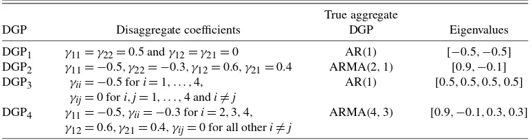
ran-dom numbers, whereν=I4. Table1summarizes the differ-ent DGPs employed in the simulations with constant parameter DGPs.
For DGP1, the parameters in (12) are γ11 =γ22 =0.5,
γ33 =γ44 =0 and γij=0 for i,j=1, . . . ,4 with i=j, so
(1+0.5L)yat =2+νt withσν2=2 for the aggregate process.
The eigenvalues of the dynamics in DGP1 are equal, and the disaggregatesy1,y2, and the aggregateyaall follow an AR(1) process, so slope misspecification will have a small effect on the relative forecast accuracy. This is the first DGP used in
Lütkepohl(1984b).
In DGP1, the direct forecast of the aggregate and aggregat-ing the disaggregate forecasts yield the same MSFE, since the components of the disaggregate multivariate process are inde-pendent and have identical stochastic structure. When the true
Table 1. Structure of DGPs for MC simulations: summary table
True aggregate
DGP Disaggregate coefficients DGP Eigenvalues
DGP1 γ11=γ22=0.5 andγ12=γ21=0 AR(1) [−0.5,−0.5] DGP2 γ11= −0.5, γ22= −0.3, γ12=0.6, γ21=0.4 ARMA(2,1) [0.9,−0.1] DGP3 γii= −0.5 fori=1, . . . ,4, AR(1) [0.5,0.5,0.5,0.5]
γij=0 fori,j=1, . . . ,4 andi=j
DGP4 γ11= −0.5, γii= −0.3 fori=2,3,4, ARMA(4,3) [0.9,−0.1,0.3,0.3]
γ12=0.6, γ21=0.4, γij=0 for all otheri=j
NOTE: DGP1, DGP2, and DGP3, DGP4are two-dimensional and four-dimensional, respectively; population variances areσvi,t=1,
i=1, . . . ,4.
model is used for estimation, the MSFE differences result only from estimation uncertainty, and not from model misspecifica-tion. Therefore, we can isolate the effect of the estimation un-certainty. The four-dimensional DGP3is constructed in a simi-lar way. DGP2differs from DGP1due to the mutual dependence of the disaggregates. Finally, we construct DGP4 to approxi-mate our empirical example of U.S. aggregate inflation: Two components are interdependent, whereas the two others behave quite differently.
The simulations were carried out based on N=1000 rep-etitions. Additional simulations for other DGPs and different sample sizes did not change the qualitative conclusions. In the paper, we only consider results forT=100 for all DGPs. All four DGPs are stationary in-sample. In DGP1 and DGP3, the aggregate process is an AR(p)model, in contrast to DGP2and DGP4where the DGPs of the aggregate are an ARMA(2,1)and ARMA(4,3)respectively. Consequently, in DGP1 and DGP3, the direct autoregressive (AR) forecast has higher accuracy rel-ative to the other methods, in contrast to DGP2and DGP4where the AR(p)model is misspecified. DGP1and DGP3have a fac-tor structure, where the facfac-tor isyawith equal weights for the disaggregates.
As inLütkepohl(1984b), we generate forecasts from inde-pendent samples. Possible extensions are to estimate the mod-els recursively, or from a rolling sample. Results based on re-cursively expanding samples for DGP1and DGP2for an initial estimation sample ofR=100 (R=200) and out-of-sample pe-riod of length P=40 (P=100) did not change the ranking of the different methods to forecast the aggregate and resulted in similar root MSFEs (RMSFEs) to independent samples (all additional results available on request).
Forecast Methods. We compare five different methods to forecast the aggregate:
1. direct forecast only using past aggregate information based on an AR model;
2. forecasting disaggregates with an AR model and aggre-gating those forecasts (indirect AR);
3. forecasting disaggregates with a VAR including all sub-components, but no aggregate information, then aggregating those forecasts (indirect VARsub);
4. forecasting disaggregates with a VAR including the ag-gregate and all subcomponents (except one to avoid collinearity when weights are constant) (direct VARagg,sub);
5. forecasting with a VAR including selected subcompo-nentsyiand the aggregate (direct VARagg,yi).
All models are estimated by (multivariate) least squares, pro-viding identical estimators to maximum likelihood under a nor-mality assumption. All simulations assume constant aggrega-tion weights, and are carried out using AIC for selecting the order of the model, since a model selection criterion would be employed in practice when the DGP is unknown.
Simulation With a Nonconstant DGP. To check analytical conclusions 1, 2, and 4 in Section2.3in small samples, we im-plemented a change in the mean and in the innovation variance as well as allowing for nonzero cross-correlations in the innova-tions in DGP1and DGP2. The change in mean is implemented by changing the intercepts of both subcomponents over the out-of-sample period (a) in the same direction for both components, and (b) in opposite directions. The change in variance is im-plemented by a change in the variance of the innovation errors over the out-of-sample period. We also carry out simulations for DGPs with different innovation variance or with different cross-correlations of the errors for the entire sample period, including both in-sample and out-of-sample. In the latter experiments we allow for positive as well as negative correlations. Throughout, we investigate the impacts of the changes on the relative rank-ings of the different methods. For comparability, we consider
T =100, independent samples, and AIC is used for lag-order selection.
3.2 Simulation Results
Constant Parameter DGP. The results are presented in Ta-bles2and3in terms of RMSFE relative to the direct AR bench-mark model. Only for the direct AR benchbench-mark actual RMSFEs are presented. Table 2 shows that for DGP1, the direct fore-cast of the aggregate based only on aggregate information is best for a 1-step ahead horizon, while the indirect forecast of the aggregate using AR models for the component forecasts is ranked second. The VAR based forecast is worst for this partic-ular DGP. The direct and indirect VAR models provide the same RMSFE because including one disaggregate component in the aggregate model when the DGP is two-dimensional is just a linear transformation of aggregating the disaggregate forecasts (see Section2.4). The simulation results for DGP1are compa-rable toLütkepohl(1987, table 5.2).
Investigating the RMSFE for all horizons between h=1 and 12 showed that the differences for horizons larger than 3 were minor, in line with the results inLütkepohl(1984b, 1987), who only presents results forh=1 andh=5. At forecast hori-zonh=12, all forecasts are almost identical. At largerT (200
Table 2. Relative RMSFE for DGP1, DGP2and DGP3,T=100
Horizon: 1 6 12
Method: Direct Indirect Direct Indirect Direct Indirect
DGP1
AR 1.408 1.010 1.634 1.006 1.656 0.999
VARsub 1.011 1.002 1.001
VARagg,sub(y1) 1.011 1.002 1.001
DGP2
AR 1.524 1.113 1.547 1.061 1.560 1.035
VARsub 0.935 0.974 0.990
VARagg,sub(y1) 0.935 0.974 0.990
DGP3
AR 2.026 1.005 2.314 1.005 2.422 1.001
VARsub 1.018 0.998 0.998
VARagg,y3 1.003 1.001 0.999
VARagg,y2,y3 1.008 0.996 0.998
NOTE: Actual RMSFE for AR model (direct) in bold. Superscripts indicate model. VARsub: VAR only including subcomponents;
VARagg,sub(yi): VAR with aggregate and subcomponenty
i. Lag order selection for all models by Akaike criterion.N=1000. See
Table1for the DGPs.
and 400, not presented), the RMSFEs of the direct and indirect forecasts of the aggregate are closer: the DGP implies equal population MSEs, so a largerT leads to a decline in both esti-mation uncertainty and lag-order selection mistakes, and there-fore higher there-forecast accuracy.
Table2, second panel, shows that for DGP2, in contrast to DGP1, the VAR forecasts are most accurate and the direct AR forecast is second best. Even though that DGP is stationary, the two eigenvalues are substantially different. For DGP2, includ-ing disaggregate information in the aggregate VAR model or forecasting the disaggregates from a VAR and aggregating their forecasts improves forecast accuracy over the other methods.
The simulation results for the four-dimensional DGP3, with independent components that have the same stochastic structure (as in DGP1), show that the direct AR forecast is again most accurate (as for DGP1), but including just one disaggregate is second best forh=1 (see Table2, third panel). For DGP4, in-stead, where the disaggregates are interdependent and follow different stochastic processes, Table3shows that including dis-aggregates in the aggregate model improves over the direct AR
forecast. The indirect VARsubprovides more accurate forecasts than the direct or indirect AR forecast forh=1.
Nonconstant Parameter DGP. The simulations investigat-ing the effects of a change in the mean and in the variance of the disaggregates on the relative forecast accuracy ranking of the different methods, yielded the following results for a one-step forecast horizon. First, a change in mean does not change the ranking of the different methods, whether the in-tercepts in the disaggregate components change in the same or in the opposite direction. This confirms our analytical re-sults in conclusion 1 in Section2.3. Second, a change in the er-ror variance of the disaggregate components out-of-sample for DGP1still leads to the same ranking of the different methods, with the AR direct having highest forecast accuracy. For DGP2 we get an unchanged ranking of the different methods. Third, changing the variances over the entire sample period, in-sample and out-of-sample, again does not alter rankings for DGP2, while for DGP1, all the RMSFEs are very close. Fourth, allow-ing for cross-correlations between innovation errors (instead of zero cross-correlations) alters the forecast accuracy ranking for
Table 3. Relative RMSFE for DGP4,T=100
Horizon: 1 6 12
Method: Direct Indirect Direct Indirect Direct Indirect
AR 2.134 1.058 2.163 0.999 2.214 1.016
VARsub 0.962 0.979 1.000
VARagg,y1 0.987 0.982 1.000
VARagg,y2 0.962 0.981 1.000
VARagg,y3 0.996 0.998 0.999
VARagg,y1,y2 0.956 0.977 1.000
VARagg,y1,y3 0.979 0.983 0.999
VARagg,y2,y3 0.957 0.981 1.000
NOTE: Actual RMSFE for AR model (direct) in bold. Superscripts indicate model. VARsub: VAR only including subcomponents; VARagg,sub(yi): VAR with aggregate and subcomponentyi. Lag order selection for all models by Akaike criterion.N=1000. See
Table1for the DGP.
DGP1, but not for DGP2. Our analytical results show that the error covariance structureper se does not affect the rankings of the different methods directly, but it does affect it indirectly through estimation uncertainty, as pointed out in conclusion 7 in Section2.3. Our simulation results confirm that in small sam-ples the error covariance structure can affect the relative estima-tion uncertainty substantively.
Summary. Overall, including disaggregate variables in the aggregate model helps forecast the aggregate if the disaggre-gates follow different stochastic structures and are interdepen-dent. The differences in forecast accuracy are less pronounced for higher horizons, since all the forecasts converge to the un-conditional mean. In particular, we find that selecting disaggre-gates helps to improve forecast accuracy by reducing estimation uncertainty if the number of disaggregates is relatively large.
4. FORECASTING AGGREGATE U.S. INFLATION
In this section, we analyze empirically the relative forecast accuracy of the three methods to forecast the aggregate, inves-tigated analytically and via Monte Carlo simulations in the pre-vious sections, for forecasting aggregate U.S. CPI inflation.
Relation to other empirical studies of contemporaneous ag-gregation and forecasting.TheIntroductiondiscusses the large empirical literature on contemporaneous aggregation and fore-casting, and the mixture of outcomes reported as to whether ag-gregation of component forecasts or forecasting the aggregate from past aggregate information alone provides the most accu-rate forecasts for aggregate inflation. For euro area countries, or the euro area as a whole, the results depend on the country analyzed, whether aggregation is considered across countries or disaggregate components, the forecasting methods or model selection procedures employed, the particular sample periods examined (e.g. before and after EMU), and the forecast hori-zons considered (see, e.g.,Marcellino, Stock, and Watson 2003;
Benalal et al. 2004;Hubrich 2005, andBruneau et al. 2007). For real U.S. GNP growth, Fair and Shiller (1990) find that disaggregate information helps forecast the aggregate, and
Zellner and Tobias (2000), find for forecasting median GDP annual growth rates of 18 industrialized countries, that fore-casts of the aggregate can be improved by aggregating disag-gregate forecasts, provided an agdisag-gregate variable is included in the disaggregate model and all coefficients are restricted to be the same across countries.
We now consider empirically two very different sample peri-ods for U.S. inflation (see, e.g.,Atkeson and Ohanian 2001and
Stock and Watson 2007for recent contributions to predictabil-ity changes in U.S. inflation). We investigate whether changes
in aggregate U.S. inflation and its components over those dif-ferent sample periods affects whether disaggregate information helps forecast the aggregate.
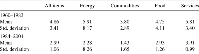
4.1 Data
The data employed in this study include the all items U.S. consumer price index (CPI) as well as its breakdown into four subcomponents: food (pf), commodities less food and energy commodities (pc), energy (pe) and services less energy services prices (ps) (Source: CPI-U for all Urban Consumers, Bureau of Labor Statistics). We employ monthly, seasonally adjusted data, except for CPI energy which does not exhibit a seasonal pattern. Seasonal adjustment by the BLS is based on X-12-ARIMA. We do not consider a real-time dataset, since revisions to the CPI in-dex are extremely small. We consider a sample period for infla-tion from 1960(1) to 2004(12), where earlier data from 1959(1) onwards are used for the transformation of the price level. As observed by other authors (e.g.,Stock and Watson 2007), there has been a substantial change in the mean and the volatility of aggregate inflation between the two samples. We document that the disaggregate components also exhibit a substantial change in mean and volatility. Aggregate as well as components of in-flation, all exhibit high and volatile behavior until the begin-ning or mid-1980s and lower, more stable rates thereafter (see Table4for details).
In Sections 4.2 and 4.3, we present results of an out-of-sample experiment for two different forecast evaluation peri-ods: 1970(1)–1983(12) and 1984(1)–2004(12). The date 1984 for splitting the sample coincides with estimates of the begin-ning of the great moderation, and is in line with what is chosen inStock and Watson(2007) andAtkeson and Ohanian(2001). We use the same split sample for comparability of our results to those studies in terms of aggregate inflation forecasts.
Due to the mixed results of ADF unit-root tests for different CPI components and samples, we carry out the forecast accu-racy comparisons for the level and the change in inflation. We present the results for the level of inflation, as results for the changes in inflation do not differ qualitatively from those for the level in terms of relative forecast accuracy of the different methods. We evaluate the 1-month-ahead and 12-month-ahead forecasts on the basis of the same forecast origin. The main cri-terion for the comparison of the forecasts here, as in a large part of the literature on forecasting, is RMSFE.
4.2 Combining Disaggregate Forecasts or Disaggregate Variables: AR and VAR Models
Forecasting Methods. We employed various forecasting methods, with different model selection procedures for both di-rect and indidi-rect forecasts (forecasting inflation didi-rectly versus
Table 4. U.S., descriptive statistics, year-on-year CPI inflation
All items Energy Commodities Food Services
1960–1983
Mean 4.86 5.91 3.80 4.75 5.81
Std. deviation 3.41 8.17 2.89 4.11 3.40
1984–2004
Mean 2.99 2.28 1.43 2.93 3.91
Std. deviation 1.06 8.26 1.65 1.26 0.99
Table 5. Relative RMSFE, U.S. year-on-year inflation (percentage points), 1970–1983
Horizon: 1 6 12
Method: Direct Indirect Direct Indirect Direct Indirect
12pˆagg 12pˆaggsub 12pˆagg 12pˆaggsub 12pˆagg 12pˆaggsub
AR 0.294 1.337 1.358 1.083 2.985 1.324
RW 1.031 1.378 1.053 1.048 1.045 1.061
MA(1) 1.395 1.198 1.899 1.828 1.695 1.318
VARsub 1.450 1.241 1.429
VARagg,sub 1.071 1.468 1.129 1.225 1.254 1.437
VARagg,f 1.046 0.992 0.936
VARagg,c 1.017 0.991 0.974
VARagg,s 1.027 0.962 0.939
VARagg,e 1.028 1.065 1.180
NOTE: Actual RMSFE (nonannualized) for direct AR model in percentage points in bold, for other models RMSFE relative to direct AR; recursive estimation samples 1960(1)to 1970(1), . . . ,1983(12); lag order selection for all models [except MA(1)model with one lag] by Akaike criterion, maximum number of lags:p=13; superscripts indicate model, VARsub: VAR only including subcomponents; VARagg,sub: VAR with aggregate and subcomponents; “direct”: direct forecast of the aggregate, “indirect”: aggregated subcomponent forecast.
aggregating subcomponent forecasts). Tables5 and 6 present the comparisons of forecast accuracy measured in terms of RMSFE of year-on-year (headline) U.S. inflation for forecast-ing aggregate (all items) inflation usforecast-ing different approaches to forecast an aggregate.
The forecasting models include: (1) a simple autoregressive (AR) model; (2) the random walk (RW) implemented as infla-tion inT+hbeing the simple average of the month-on-month inflation rate from T−12 toT, as used in Stock and Watson
(2007) referring toAtkeson and Ohanian(2001); (3) a subcom-ponent VARsubto indirectly forecast the aggregate by aggregat-ing subcomponent forecasts; (4) VARs includaggregat-ing the aggregate and all disaggregate components (perfect collinearity between aggregate and components does not occur due to annually changing weights in price indices), or a selected number of dis-aggregate components, VARagg,suband VARagg,subi; and (5) an
MA(1)(as used in Stock and Watson 2007). Results for fac-tor models are presented in the next section. Model selection procedures selecting the lag length in the various models em-ployed above include the Schwarz (SIC) and the Akaike (AIC) criterion, respectively, with maximum lag order of 13. We find
that the AIC-based models generally perform better for U.S. inflation and therefore present results for those models.
The benchmark model for the comparison is the (direct) fore-cast of aggregate inflation from the AR model, simply forefore-cast- forecast-ing aggregate inflation from its own past (first entry in column labeled “direct” in Tables5and6). This is compared to the in-direct forecast from the AR model, that is, the aggregated AR forecasts of the subindices, as well as to the other methods of forecasting the aggregate directly (column labeled “direct”) or indirectly (column labeled “indirect”) using VARs (see above). The combination of the disaggregate forecasts for all models is implemented by replicating the aggregation procedure em-ployed by the BLS for the CPI disaggregate data. The data are aggregated in levels, taking into account the respective base year of the weights. Historical aggregation weights were pro-vided to the authors by the BLS. For the aggregation of the forecasts, the current aggregation weights are used, since future weights would not be known to the forecaster in real time.
12pˆagg and12pˆaggsub indicate that the forecast is evaluated on the basis of year-on-year inflation. The models are, how-ever, specified in terms of month-on-month inflation. It should be noted that the ranking of the different forecast methods is
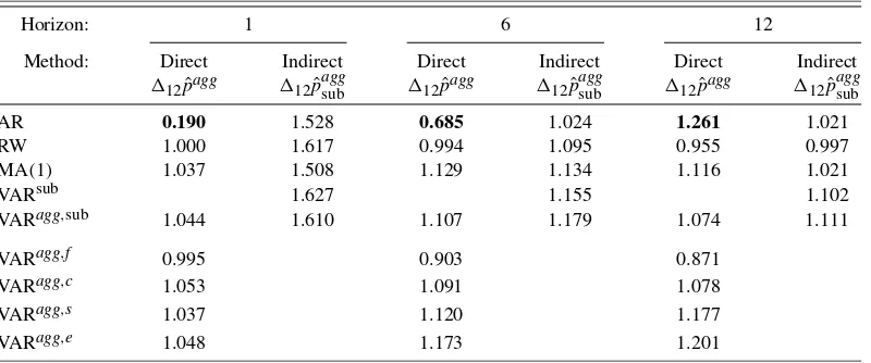
Table 6. Relative RMSFE, U.S. year-on-year inflation (percentage points), 1984–2004
Horizon: 1 6 12
Method: Direct Indirect Direct Indirect Direct Indirect
12pˆagg 12pˆaggsub 12pˆagg 12pˆaggsub 12pˆagg 12pˆaggsub
AR 0.190 1.528 0.685 1.024 1.261 1.021
RW 1.000 1.617 0.994 1.095 0.955 0.997
MA(1) 1.037 1.508 1.129 1.134 1.116 1.021
VARsub 1.627 1.155 1.102
VARagg,sub 1.044 1.610 1.107 1.179 1.074 1.111
VARagg,f 0.995 0.903 0.871
VARagg,c 1.053 1.091 1.078
VARagg,s 1.037 1.120 1.177
VARagg,e 1.048 1.173 1.201
NOTE: As Table5, but recursive estimation samples 1960(1)to 1984(1), . . . ,2004(12).
not invariant to the selected transformations (see, e.g.,Clements and Hendry 1998, p. 68). We found that models formulated in terms of year-on-year inflation provided the same ranking and less accurate forecasts than those for monthly changes in in-flation evaluated at year-on-year inin-flation. Iterative multistep ahead forecasts are based on the following model (only includ-ing one lag of inflation and no other macroeconomic variables as predictors for expositional purposes):πˆT+h= ˆαhi=0−1βˆi+
ˆ
βhπT, where inflation πt is specified in first differences as
(Pt−Pt−1)/Pt−1. Results for the change in inflation were not qualitatively different from the results for the level of inflation. In the tables values below unity for the relative RMSFE indicate an improvement in that forecast over the direct AR forecast.
Results. The RMSFE results indicate, first, that the direct forecast is generally more accurate than the indirect forecast of the aggregate, irrespective of whether disaggregate informa-tion is included in the aggregate model or not. Second, for the high inflation sample in the 1970s, including one disaggregate in the aggregate model might improve over the direct AR model forecast for longer horizons as well as over the MA(1). The MA(1)is less accurate than the AR(p)in the first sample pe-riod and similar to it in the second (seeStock and Watson 2007, who analyze four different price measures, for similar results for quarterly CPI inflation). Including disaggregate variables in most cases also dominates combining disaggregate forecasts in RMSFE terms. For the latter sample 1984–2004, including food inflation in the aggregate model improves forecast accu-racy over the direct AR model for all horizons. Interestingly, including food inflation in the aggregate model also improves over the RW model that performs better in RMSFE terms for the second sample period for a one-year horizon. It also im-proves over the MA(1) for all horizons. We apply theClark and West(2007) test of equal forecast accuracy for the food in-flation model against an AR benchmark for a horizon of one month, and find that this RMSFE improvement is significant at the 10% level. It should be noted, however, that the improve-ment is not significant when using appropriate critical values for testing a set of four models including different disaggre-gates against the benchmark AR model for the aggregate (see
Hubrich and West 2010, also for similar results for other macro-economic regressors). Overall, the results suggest that variable selection is important in reducing the impact of parameter un-certainty here.
4.3 Disaggregate Information in Dynamic Factor Models
We now compare combining disaggregate information by in-cluding factors estimated from the disaggregate components in the aggregate model with forecasting the aggregate by the benchmark AR model. The analytical investigation showed es-timation uncertainty to be an important determinant of the rel-ative forecast accuracy of the different methods to forecast an aggregate. Factor models can reduce estimation uncertainty in comparison with a VAR with many parameters. We employ fac-tor models averaging away idiosyncratic variation in the disag-gregate series, and include the factors, estimated by principal components from disaggregate price information, in the aggre-gate model.
Under the assumptions inStock and Watson(2002a, 2002b) the model is identified and the factors and loadings can be estimated. Related studies of approximate factor models have shown consistency of principal components estimators of the factor space, for example,Bai(2003),Bai and Ng(2002), and
Forni et al.(2000, 2005). Treatments of classical factor mod-els when the cross-sectional dimensionnis small can be found in, for example,Anderson(1984),Geweke(1977),Sargent and Sims (1977), and Stock and Watson (1991). A larger cross-section relative toTimproves asymptotic performance, in that consistency is achieved at a faster rate compared to a small cross-section (see Stock and Watson 1998). To keep our in-formation set comparable with that in the forecast experiments with VAR models, we retained the same disaggregate variables. Little is known so far how the size and the composition of the data affect the factor estimates (see, e.g.,Boivin and Ng 2006). We are concerned with how factors from disaggregate informa-tion affect forecast accuracy of the aggregate economic vari-able. Since the models considered here are more parsimonious than many VARs considered above, forecast accuracy may be less affected by estimation uncertainty.
The results from the factor analysis are not directly compara-ble across all horizons with previous tacompara-bles except forh=12, since here direct multistep ahead forecasts are carried out and forecast accuracy is evaluated for annualized inflation in line withStock and Watson(1999, 2007) (instead of year-on-year inflation as above). We compute the directh-step factor fore-casts and single predictor forefore-casts, and consider forecast com-binations of all single predictor models based on the respec-tive disaggregate component with equal weights. The results are presented in Table7.
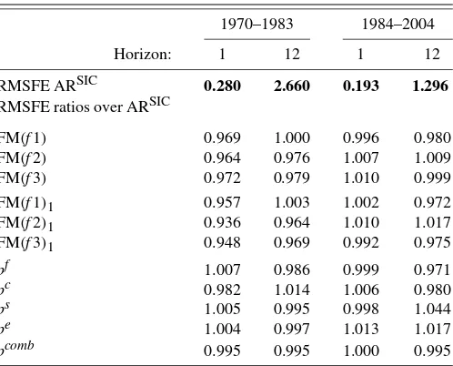
For the first sample, disaggregate information helps forecast aggregate U.S. inflation one and 12 months ahead. The im-provements over the AR model are up to 6.5% in RMSFE terms
Table 7. U.S., RMSFE ratios
1970–1983 1984–2004
Horizon: 1 12 1 12
RMSFE ARSIC 0.280 2.660 0.193 1.296
RMSFE ratios over ARSIC
FM(f1) 0.969 1.000 0.996 0.980
pf 1.007 0.986 0.999 0.971
pc 0.982 1.014 1.006 0.980
ps 1.005 0.995 0.998 1.044
pe 1.004 0.997 1.013 1.017
pcomb 0.995 0.995 1.000 0.995
NOTE: RMSFE (not annualized) for AR(SIC) model in percentage points; SIC: lag order selection by Schwarz criterion; Recursive estimation samples 1960(1) to 1970(1), . . . ,1983(12)and 1960(1)to 1984(1), . . . ,2004(12); FM(fi): factor models with
i=1,2,3 static factors; FM(fi)1: factor models withi=1,2,3 factors with 1 lag;
prin-cipal component estimators of static factors;pf,pc,ps,pe: single predictor models with
respective subcomponent as predictor;pcomb: simple average of the forecasts from the four disaggregate component models.
(up to 12.5% in MSFE terms). Including one factor is statis-tically significant for the first sample period for a one-month horizon by theClark and West(2007) test of equal forecast ac-curacy. However, the improvement using factor models is lower in the second sample period. This is in line with whatStock and Watson(2007) find for including real variables in an inflation model.
4.4 Summary of Empirical Results
To summarize our empirical results, overall the direct fore-cast of the aggregate, either using only past aggregate or using disaggregate information, is more accurate than combining dis-aggregate forecasts. Therefore, combining disdis-aggregate infor-mation helps over combining disaggregate forecasts. Further, including a selected number of disaggregate variables or factors summarizing disaggregate information tends to improve fore-cast accuracy over forefore-casting the aggregate directly by only using past aggregate information, in particular in samples with sufficient variability in the aggregate.
5. CONCLUSIONS
We presented new analytical results on the relative forecast accuracy of forecasting an aggregate by (1) combining disag-gregate forecasts (forecasting the disagdisag-gregate variables then aggregating those forecasts), (2) using only lagged aggregate information, and (3) to combine disaggregate information by including a subset of disaggregate components (or a combina-tion thereof) in the aggregate model.
In the analytical derivations we investigated the effects of misspecification and estimation uncertainty on the relative fore-cast accuracy of the three different approaches to forefore-casting an aggregate, and we extended previous results by allowing for a change in the parameters of the DGP unknown to the forecaster, forecast origin uncertainty and time-varying weights. Decom-positions of the sources of forecast errors led us to conclude that relative forecast accuracy is not affected by forecast-origin location shifts and slope changes, whereas absolute accuracy is. This is in contrast to the forecast combination literature, which focuses on combining forecasts of the same variable, where combination helps in the presence of mean shifts in opposite directions. Our second main result, in addition to a number of other important conclusions, is that slope misspecification and estimation uncertainty are the primary sources of differences in forecast accuracy between the different methods.
In the Monte Carlo simulations we find that including dis-aggregate variables in the dis-aggregate model helps forecast the aggregate if the disaggregates follow different stochastic struc-tures, the components are interdependent, and only a selected number of components is included to reduce estimation uncer-tainty. Unknown and unmodeled structural change in the mean does not affect relative forecast error of the different forecast methods, even though it has major effects on absolute forecast accuracy.
The empirical results for U.S. CPI inflation before and af-ter the Great Moderation confirmed our analytical and simu-lation findings that estimation uncertainty plays an important role in relative forecast accuracy across the different approaches
to forecast an aggregate. Consequently, we recommend model selection procedures for choosing the disaggregates to be in-cluded in the aggregate model, or methods to combine disag-gregate information, and careful modeling of location shifts. Alternative methods for reducing estimation uncertainty, such as Bayesian or shrinkage methods, are beyond the scope of the paper, but are an interesting direction of further research in this context.
APPENDIX: FORECAST ERROR
DECOMPOSITION—ADDITIONAL DERIVATIONS
The decomposition for the long-run mean, the first bracketed term in (5), is
ω′φ∗y−ω′φˆy=ω′(φy∗−φy)+ω′(φy−φy,e)
+ω′(φy,e− ˆφy). (A.1) Decomposingω′Ŵˆ(yˆT − ˆφy)=ω′Ŵˆ(yˆT−yT)+ω′Ŵˆ(yT− ˆφy)
to separate the measurement error, the second bracketed term in (5), becomes ω′Ŵ∗(yT −φ∗y)−ω′Ŵˆ(yT − ˆφy) and can be
decomposed as
−ω′(Ŵ∗−Ŵ)(φ∗y−φy)−ω′(Ŵ−Ŵe)(φ∗y−φy)
−ω′Ŵe(φ∗y−φy)+ω′(Ŵ∗−Ŵ)(yT−φy)
+ω′(Ŵ−Ŵe)(yT−φy)−ω′Ŵe(φy−φy,e)
−ω′(Ŵˆ −Ŵe)(yT−φy)−ω′(Ŵˆ−Ŵe)(φy−φy,e)
+ω′Ŵe(φˆy−φy,e)+ω′(Ŵˆ−Ŵe)(φˆy−φy,e). (A.2)
ω′Ŵˆ(yˆT −yT)can be decomposed, such that collecting terms
from (A.1) and (A.2) above yields the taxonomy in (6).
ACKNOWLEDGMENTS
We thank Marcel Bluhm and Eleonora Granziera for excel-lent research assistance. We thank two anonymous referees, an associate editor, and the editor Arthur Lewbel for valuable comments. We are grateful to Olivier de Bandt, Domenico Gi-anonne, Lutz Kilian, Helmut Lütkepohl, Serena Ng, Lucrezia Reichlin, Kenneth West, and seminar participants at Bocconi University, Duke University, the Federal Reserve Bank of At-lanta, the Federal Reserve Board, the University of Michigan, the University of Wisconsin, participants of the EUI Confer-ence 2006, ISF 2007, NASM 2007, and EABCN-CEPR con-ference 2007 for useful comments. We thank Walter Lane and Patrick Jackman (BLS) for providing the historical weights for the U.S. CPI data. Financial support from the ESRC under grant RES 051 270035 is gratefully acknowledged. The views ex-pressed in this paper are not necessarily those of the European Central Bank.
[Received May 2007. Revised April 2009.]
REFERENCES
Anderson, T. W. (1984),An Introduction to Multivariate Statistical Analysis
(2nd ed.), New York: Wiley. [225]
Atkeson, A., and Ohanian, L. E. (2001), “Are Phillips Curves Useful for Fore-casting Inflation?”Federal Reserve Bank of Minneapolis Quarterly Review, 25 (1), 2–11. [223,224]
Bai, J. (2003), “Inference on Factor Models of Large Dimensions,” Economet-rica, 71 (1), 135–172. [225]
Bai, J., and Ng, S. (2002), “Determining the Number of Factors in Approximate Factor Models,”Econometrica, 70 (1), 191–221. [225]
Benalal, N., del Hoyo, J. L. D., Landau, B., Roma, M., and Skudelny, F. (2004), “To Aggregate or Not to Aggregate? Euro Area Inflation Forecasting,” Working Paper 374, European Central Bank. [216,223]
Bernanke, B. (2007), “Inflation Expectations and Inflation Forecasting,” speech at the Monetary Economics Workshop of the NBER Summer Institute. Available at http:// www.federalreserve.gov/ newsevents/ speech/
Bernanke20070710a.htm. [216]
Boivin, J., and Ng, S. (2006), “Are More Data Always Better for Factor Analy-sis?”Journal of Econometrics, 132, 169–194. [225]
Bruneau, C., De Bandt, O., Flageollet, A., and Michaux, E. (2007), “Forecast-ing Inflation Us“Forecast-ing Economic Indicators: The Case of France,”Journal of Forecasting, 26, 1–22. [216,223]
Carson, R., Cenesizoglu, T., and Parker, R. (2007), “Aggregation Issues in Forecasting Aggregate Demand: An Application to US Commercial Air Travel,” unpublished manuscript, University of California. Available at
http:// ssrn.com/ abstract=1401453. [217]
Clark, T. E., and McCracken, M. W. (2006), “Forecasting With Small Macro-economic VARs in the Presence of Instabilities,” Research Working Pa-per 06-09, The Federal Reserve Bank of Kansas City. [217]
Clark, T. E., and West, K. D. (2007), “Approximately Normal Tests for Equal Predictive Accuracy in Nested Models,”Journal of Econometrics, 138 (1), 291–311. [225,226]
Clements, M. P., and Hendry, D. F. (1998),Forecasting Economic Time Series, Cambridge, U.K.: Cambridge University Press. [217,218,225]
(1999), Forecasting Non-Stationary Economic Time Series, Cam-bridge, MA: MIT Press. [217]
(2004), “Pooling Forecasts,”Econometrics Journal, 7, 1–31. [219] (2006), “Forecasting With Breaks in Data Processes,” inHandbook of Economic Forecasting, eds. G. Elliott, C. W. J. Granger, and A. Timmer-mann, Amsterdam, Netherlands: Elsevier, pp. 605–657. [217,218] Elliott, G. (2007), “Unit Root Pre-Testing and Forecasting,” mimeo,
Univer-sity of California, San Diego. Available athttp:// www-leland.stanford.edu/
group/ SITE/ archive/ SITE_2006/ Web%20Session%205/ Elliott.pdf. [218]
Espasa, A., Senra, E., and Albacete, R. (2002), “Forecasting Inflation in the European Monetary Union: A Disaggregated Approach by Countries and by Sectors,”European Journal of Finance, 8 (4), 402–421. [216] Fair, R. C., and Shiller, J. (1990), “Comparing Information in Forecasts From
Econometric Models,”The American Economic Review, 80 (3), 375–389. [216,223]
Forni, M., Hallin, M., Lippi, M., and Reichlin, L. (2000), “The Generalized Fac-tor Model: Identification and Estimation,”Review of Economics and Statis-tics, 82, 540–554. [225]
(2005), “The Generalized Factor Model: One-Sided Estimation and Forecasting,”Journal of the American Statistical Association, 100 (471), 830–840. [225]
Garderen, V. K. J., Lee, K., and Pesaran, M. H. (2000), “Cross-Sectional Ag-gregation of Non-Linear Models,”Journal of Econometrics, 95, 285–331. [216]
Geweke, J. F. (1977), “The Dynamic Factor Analysis of Economic Time Se-ries,” inLatent Variables in Socio-Economic Models, eds. D. J. Aigner and A. S. Goldberger, Amsterdam: North-Holland. [225]
Giacomini, R., and Granger, C. W. J. (2004), “Aggregation of Space-Time Processes,”Journal of Econometrics, 118, 7–26. [216,217,220]
Granger, C. (1987), “Implications of Aggregation With Common Factors,”
Econometric Theory, 3, 208–222. [216,217]
Granger, C. W. J. (1980), “Long Memory Relationships and the Aggregation of Dynamic Models,”Journal of Econometrics, 14, 227–238. [217] Grunfeld, Y., and Griliches, Z. (1960), “Is Aggregation Necessarily Bad?”The
Review of Economics and Statistics, 42 (1), 1–13. [216]
Hendry, D. F., and Hubrich, K. (2006), “Forecasting Aggregates by Disaggre-gates,” Working Paper 589, European Central Bank. [217]
Hernandez-Murillo, R., and Owyang, M. T. (2006), “The Information Content of Regional Employment Data for Forecasting Aggregate Conditions,” Eco-nomics Letters, 90, 335–339. [217]
Hubrich, K. (2005), “Forecasting Euro Area Inflation: Does Aggregating Fore-casts by HICP Component Improve Forecast Accuracy?” International Journal of Forecasting, 21 (1), 119–136. [216,217,223]
Hubrich, K., and West, K. (2010), “Forecast Evaluation of Small Nested Model Sets,”Journal of Applied Econometrics, to appear. [225]
Kohn, R. (1982), “When Is an Aggregate of a Time Series Efficiently Forecast by Its Past?”Journal of Econometrics, 18, 337–349. [216,217]
Lütkepohl, H. (1984a), “Linear Transformations of Vector ARMA Processes,”
Journal of Econometrics, 26, 283–293. [217]
(1984b), “Forecasting Contemporaneously Aggregated Vector ARMA Processes,”Journal of Business & Economic Statistics, 2 (3), 201–214. [216,217,220,221]
(1987),Forecasting Aggregated Vector ARMA Processes, Berlin, Ger-many: Springer-Verlag. [216,220,221]
(2006), “Forecasting With VARMA Processes,” inHandbook of Eco-nomic Forecasting, eds. G. Elliott, C. W. J. Granger, and A. Timmermann, Amsterdam, Netherlands: Elsevier. [216]
Marcellino, M., Stock, J. H., and Watson, M. W. (2003), “Macroeconomic Fore-casting in the Euro Area: Country Specific versus Area-Wide Information,”
European Economic Review, 47, 1–18. [216,223]
Moser, G., Rumler, F., and Scharler, J. (2007), “Forecasting Austrian Inflation,”
Economic Modelling, 24, 470–480. [216]
Pesaran, M. H., Pierse, R. G., and Kumar, M. S. (1989), “Econometric Analysis of Aggregation in the Context of Linear Prediction Models,”Econometrica, 57, 861–888. [216]
Reijer, A., and Vlaar, P. (2006), “Forecasting Inflation: An Art as Well as a Science!”De Economist, 127 (1), 19–40. [216]
Sargent, T. J., and Sims, C. A. (1977), “Business Cycle Modeling Without Pre-tending to Have Too Much a-priori Theory,” inNew Methods in Business Cycle Research, ed. C. Sims, Minneapolis: Federal Reserve Bank of Min-neapolis. [225]
Stock, J. H., and Watson, M. W. (1991), “A Probability Model of the Co-incident Economic Indicator,” inThe Leading Economic Indicators: New Approaches and Forecasting Records, eds. G. Moore and K. Lahiri, Cam-bridge, U.K.: Cambridge University Press, pp. 63–90. [225]
(1996), “Evidence on Structural Instability in Macroeconomic Time Series Relations,”Journal of Business & Economic Statistics, 14 (1), 11– 30. [217]
(1998), “Diffusion Indexes,” Working Paper 6702, NBER. [225] (1999), “Forecasting Inflation,”Journal of Monetary Economics, 44, 293–335. [225]
(2002a), “Forecasting Using Principal Components From a Large Number of Predictors,”Journal of the American Statistical Association, 97, 1167–1179. [225]
(2002b), “Macroeconomic Forecasting Using Diffusion Indices,” Jour-nal of Business & Economic Statistics, 20 (2), 147–162. [225]
(2007), “Why Has U.S. Inflation Become Harder to Forecast?”Journal of Money, Credit and Banking, 39, 3–34. [217,223-226]
Zellner, A., and Tobias, J. (2000), “A Note on Aggregation, Disaggregation and Forecasting Performance,”Journal of Forecasting, 19, 457–469. [216,217,
223]