T H E J O U R N A L O F H U M A N R E S O U R C E S • 46 • 1
Pensions and Household Wealth
Accumulation
Gary V. Engelhardt
Anil Kumar
A B S T R A C T
Economists have long suggested that higher private pension benefits “crowd out” other sources of household wealth accumulation. We exploit detailed information on pensions and lifetime earnings for older workers in the 1992 wave of the Health and Retirement Study and employ an in-strumental-variable (IV) identification strategy to estimate crowd-out. The IV estimates suggest statistically significant crowd-out: each dollar of pen-sion wealth is associated with a 53–67 cent decline in nonpenpen-sion wealth. With less precision, we use an instrumental-variable quantile regression es-timator and find that most of the effect is concentrated in the upper quan-tiles of the wealth distribution.
I. Introduction
Economists have long suggested that higher private pension benefits “crowd out” other sources of household wealth accumulation. If so, then the ability of the government to raise overall household and national saving through pension and tax policies may be limited. While there has been substantial interest in the extent to which targeted savings incentives, such as 401(k) plans and Individual
Gary V. Engelhardt is a professor in the Department of Economics and Center for Policy Research in the Maxwell School of Citizenship and Public Affairs of Syracuse University. Anil Kumar is a senior economist in the regional group of the Federal Reserve Bank of Dallas. All research with the restricted-access data from the Health and Retirement Study was performed under agreement in the Center for Policy Research at Syracuse University and the Federal Reserve Bank of Dallas. The authors thank Rob Alessie, Dan Black, Raj Chetty, Chris Cunningham, Alan Gustman, Jeff Kubik, Annamaria Lusardi, Tim Smeeding, and seminar participants at NETSPAR, Rand Corporation, and Syracuse University for help-ful discussions and comments. They are especially gratehelp-ful to Bob Peticolas and Helena Stolyarova for their efforts in helping us understand the HRS employer-provided pension plan data. They thank the TIAA-CREF Institute for graciously supporting this research. The opinions and conclusions are solely those of the authors and should not be construed as representing the opinions or policy of any agency of the Federal Reserve, TIAA-CREF, or Syracuse University. The authors claim all errors as their own. The data used in this article can be obtained beginning from August 2011 through July 2014 from Gary V. Engelhardt, 423 Eggers Hall, Syracuse University, Syracuse, NY, 13244, gvengelh@maxwell.syr.edu.
[Submitted April 2009; accepted December 2009]
Retirement Accounts (IRAs), raise retirement saving, there have been comparatively fewer studies of the extent of crowd-out across all private pension types in the United States, and the empirical evidence is mixed.1Since the seminal time-series studies of Feldstein (1974, 1996), a series of cross-sectional household studies, most notably Gale (1998), have suggested large offsets of 50 cents to one dollar of nonpension wealth with respect to each dollar of private pension wealth.2 In contrast, other studies suggested much smaller offsets of 0–33 cents.3This wide range of estimates likely reflects a variety of differences in empirical methodology across studies, in-cluding the time period, household survey, measurement of pension wealth and life-time earnings, and, perhaps most importantly, the approach to econometric identi-fication.
There are four problems that plague identification in this literature. First, pension wealth may be measured with error, which would impart bias to empirical studies of the effect of pensions on saving. Second, for many pension plans, demographics, employment characteristics, and career earnings map into benefits in a nonlinear manner. If these factors also independently affect nonpension wealth accumulation nonlinearly, then estimates of pension crowd-out will suffer from omitted-variable bias. Third, the presence of unobserved heterogeneity in household saving behavior can bias crowd-out estimates. In particular, some households may have a high taste for saving (patience). These households may accumulate more wealth in all forms, including pensions, so that it is difficult to identify the impact of pensions on non-pension wealth separately from tastes for saving. The presence of such heterogeneity would bias upward standard Ordinary Least Squares (OLS) estimates of the pension offset, toward an estimated offset that is too small, perhaps suggesting little crowd-out. This may be compounded by the fact that these households may also have higher lifetime earnings—if patient individuals invest in human capital to a greater degree—which also are correlated with pension benefits, yet most household surveys do not measure career or lifetime earnings, a key explanatory variable in crowd-out specifications. Finally, workers may sort to jobs based on pension generosity, which is another dimension on which unobserved heterogeneity might bias crowd-out es-timates.
In this paper, we depart from the recent literature focused on the specific effects of targeted subsidies to saving, such as 401(k)s and IRAs, and give new estimates of crowd-out across all pension types. Specifically, we exploit detailed administrative data on pensions and lifetime earnings for older workers in the 1992 wave of the Health and Retirement Study (HRS) and an instrumental-variable (IV) approach to attempt to circumvent these difficulties and identify the extent to which pension wealth crowds out nonpension wealth.
1. Studies on targeted saving incentives include Poterba, Venti, Wise (1995, 1996), Hubbard and Skinner (1996), Engen, Gale and Scholz (1996), Madrian and Shea (2001), Choi, Laibson, Madrian, and Metrick (2002, 2003, 2004), Choi, Laibson, and Madrian (2004), Duflo, Gale, Liebman, Orszag, and Saez (2006). 2. For example, Munnell (1974, 1976), Feldstein and Pellechio (1979), Diamond and Hausman (1984), and, more recently, Khitatrakun, Kitamura and Scholz (2001).
Engelhardt and Kumar 205
Our primary innovation is to use employer-provided pension Summary Plan De-scriptions (SPDs)—legal deDe-scriptions of pensions written in plain English—matched to HRS respondents, in conjunction with detailed pension-benefit calculators, to con-struct an instrumental variable for self-reported pension wealth under the assumption that any error in SPD-based pension wealth is uncorrelated with measurement error in self-reported pension wealth. The basic idea is similar in spirit to that used in studies by Kane, Rouse, and Staiger (1999) and Berger, Black, and Scott (2000), who have estimated the return to schooling in the presence of measurement error when there are two measures of years of education, one self-reported and one ad-ministrative (such as transcript data). To help ensure that the SPD-based instrument is uncorrelated with household-level heterogeneity and omitted variables that are nonlinear functions of individual demographics, employment characteristics, and earnings, we construct the instrument using a fixed set of demographic and employ-ment characteristics and sample mean earnings. When this is done, the variation in our instrument is due to cross-plan differences in generosity, not to worker charac-teristics that independently might determine nonpension wealth accumulation.
Two excellent recent studies by Attanasio and Brugiavini (2003) and Attanasio and Rohwedder (2003) have formed instrumental variables by exploiting plausibly exogenous national policy changes to circumvent the identification concerns outlined above and estimate pension-saving offsets in Italy and the United Kingdom, respec-tively. Our paper is methodologically different than these studies and, to the best of our knowledge, is the first to use instrumental-variable techniques to attempt to identify the extent of pension crowd-out in the United States.
We employ two additional empirical innovations. To help circumvent difficulties with measuring lifetime earnings that have plagued many previous studies, we use administrative data for HRS respondents from two sources: W-2 earnings records for 1980–91 provided by the Internal Revenue Service (IRS) and Social Security covered earnings records for 1951–91 from the Social Security Administration (SSA). In addition, we use the Instrumental Variable Quantile Regression (IVQR) estimator of Chernozhukov and Hansen (2004, 2005) to examine crowd-out at dif-ferent points in the nonpension wealth distribution.
We have three primary findings. First, our estimates of crowd-out suggest that each dollar of pension wealth is associated with 53–67 cents less in nonpension wealth. Second, the OLS estimates are biased upward, so much so that they indicate that pension wealthcrowds innonpension wealth accumulation by 23 cents. About one-half of the difference between the OLS and IV estimates can be attributed to bias from measurement error, with the other half due to nonlinearities and unmea-sured heterogeneity. Finally, with less precision than the IV results, the IVQR esti-mates suggest considerable differences in crowd-out at different points in the non-pension wealth distribution: no crowd-out at or below the median, but crowd-out of 30–75 cents in the upper quantiles.
This study is organized as follows. In Section II, we describe the HRS data on pensions and earnings. Section III discusses the regression specification, identifica-tion, and baseline estimates. Section IV presents extensions and robustness checks, and Section V presents additional results that suggest sorting is not confounding our IV estimates. The sixth section discusses the IVQR results. There is a brief conclu-sion.
II. Data Description
We use detailed data from the first wave of the HRS, a nationally representative random sample of 51–61 year olds and their spouses (regardless of age), which asked about wealth, income, demographics, and employment in 1992. Questions on employment were asked for the job (if any) held at the time of the interview, referred to hereafter as the “current job,” as well as up to three previous jobs that lasted five years or longer. For each of these jobs, individuals were asked first if they were included in a pension, retirement, or tax-deferred savings plan. We consider those who answered “yes” to be in pension-covered employment on that job. In addition, we consider those who indicated that they were eligible for, but not participating in a plan, to be pension-covered.
For those included in a plan, the survey followed up with a question about plan type for each plan (up to three plans) for that job: formula-based or defined benefit (DB) plan; account-based or defined contribution (DC) plan; or a combination plan (with a mix of DB and DC features). Based on the answer, respondents were routed through different question sequences, one for DBs, one for DCs, and one for com-bination plans, with each sequence asking about features unique to that plan type, for example, plan balances, number of years included in the plan, the amount of the employer contribution, the amount of the employee contribution, etc., for DC plans, and early and normal retirement dates, number of years in the plan, expected benefits, etc., for DB plans. The respective responses allow for the calculation of pension wealth for each plan type that then can be summed across plans for each job to yield a pension-wealth measure for the job.
A unique feature of the HRS is that the study used the job rosters from the interviews and attempted to collect SPDs from employers of HRS respondents for all current and previous jobs in which the respondent was covered by a pension. We use these to form our instrument, detailed in the next section.
Engelhardt and Kumar 207
There are a number of important reasons for the failure to match an SPD to the respondent. The respondent may not have given the correct employer name and address. Alternatively, the HRS may have failed to receive the SPD because the employer may not have complied with the pension-provider survey, the employer could not be located at the address given, or the employer went out of business or merged with another company and no longer existed under the name given by the respondent. Finally, the employer may have submitted an SPD, but the HRS was unable to match the SPD to the respondent based on the plan detail and the respon-dent’s characteristics. For these reasons, the subgroup of individuals in pension-covered employment with an associated SPD may be nonrandom, a point to which we return below.
A total of 5,607 households have an individual employed at the time of the in-terview. In the next section, we estimate crowd-out on the subsample of 2,728 house-holds who either were working but not in a pension-covered current job, or were in a pension-covered current job and had a matched SPD. Therefore, the 2,879 house-holds (that is, 2,879⳱5,607ⳮ2,728) who are omitted are those who were in a pension-covered current job, but for whom the HRS failed to match an SPD. Hence, selection bias is a potential problem for our sample.
As an important contribution of this paper is the instrumental-variable strategy for the pension-wealth estimation based on the SPDs, and the highest SPD rate was for current jobs (65 percent), we focus on those with current jobs. Due to the age-based sampling frame of the HRS, respondents’ current jobs are likely to be their career jobs, which generate the bulk of their lifetime private pension benefits (Gust-man and Steinmeier 1999).
Finally, in addition to the extensive pension data, the HRS asked respondents’ permission to link their survey responses to administrative earnings data from SSA and IRS. These administrative data include Social Security covered-earnings histo-ries from 1951–91 and W-2 earnings records for jobs held from 1980–91, and were made available for use under a restricted-access confidential data agreement. These data are the basis for our measure of lifetime earnings.
III. Regression Specification, Identification, and
Estimation Results
Let i index the household, then to determine the extent of crowd-out, we estimate the following econometric specification:
ˆ W⳱PⳭYiⳭ␣xⳭ␥ⳭⳭu
(1) i i i i i i
in which the dependent variable,W, is nonpension household net worth, andPand are functions of pension wealth and lifetime earnings, respectively. The specifi-Y
cation includes a vector of variables that proxy for future earnings, , plus a set ofx controls for demographic and employment characteristics, , and the disturbance term, .u4The estimated selection-correction term, , accounts for the possibility thatˆ
those with a matched SPD are not a random sample of pension-covered workers. The primary objective is to obtain consistent estimates of, the impact of an ad-ditional dollar of pension wealth on nonpension wealth, holding lifetime earnings and other factors constant.
A. Variable Definitions
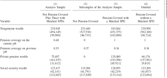
Column 1 of Table 1 shows the means for the primary variables used in the empirical analysis, with standard deviations in parentheses, and medians in square brackets, for the analysis sample. Columns 2 and 3 show similar statistics for the two sub-samples: those not in a pension-covered current job and those in a pension-covered current job with an associated SPD, respectively. Column 4 shows statistics for the omitted observations, described in the previous section—people who were in a pen-sion-covered current job, but for whom there are no associated SPDs.
The outcome variable of interest is W, nonpension household net worth, and is defined as the sum of cash, checking and saving accounts, certificates of deposit, IRAs, stocks, bonds, owner-occupied housing, business, other real estate, vehicle net equity, and other assets less other debts, and includes imputed values based on HRS public-use imputations of missing asset and debt information taken from the HRS website. The sample mean nonpension wealth is $220,000. However, the median was $95,000, which illustrates the well-known fact that the distribution of wealth is right-skewed.
The variable Y is a function of the present value of lifetime earnings for the household. As already described, we use administrative earnings data from SSA and IRS that include Social Security covered-earnings histories from 1951–91 and W-2 earnings records for jobs held from 1980–91 to construct this measure. The details are described in the appendix.
The vector xaccounts for factors that affect the present value of future earnings. It contains indicator variables for whether the head and spouse, respectively, ex-pected real earnings growth in the future, based on the following HRS question,
“Over the next several years, do you expect your earnings, adjusted for inflation, to go up, stay about the same, or go down?”
This variable takes on a value of zero if the individual expected real earnings to stay the same and one if the individual expected real earnings to go up. Similarly, we define a dummy variable for whether the head (spouse) expects real earnings to decline. In addition,xcontains a quartic in the ages of the head and spouse, expected ages at retirement of the head and spouse, current earnings of the head and spouse, interactions of the age quartics with education and current earnings, the region of birth for the respondent and spouse, and a constant.
Engelhardt and Kumar 209
employment controls are dummy variables for union status, firm-size category, and Census region.
The focal explanatory variable is P, which is a function of pension wealth, and is defined as the sum of two components. Its basis is self-reported private pension wealth calculated by Venti and Wise (2001). Because some private pensions are structured so that their benefits are integrated with Social Security benefits, we also include Social Security wealth, as constructed by Mitchell, Olson, and Steinmeier (1996) and Gustman, Mitchell, Samwick, and Steinmeier (1999), in our measure of , so that hereafter “self-reported pension wealth” refers to the sum of public and P
private pension wealth.Pis constructed to take into account the time the household has had since the introduction of each pension plan to adjust the lifetime consump-tion stream using Gale’sQ(Gale 1998). This is detailed in the appendix as well.
Overall, the analysis sample consists of mostly white, married individuals in their mid-50s, with some college education and relatively few children at home. Only 57 percent of the sample was employed in a current pension-covered job in 1992. B. OLS Estimates
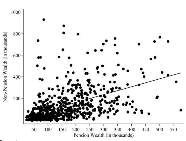
In Figure 1, we collapse the analysis sample into age⳯education⳯race⳯marital status cells and plot nonpension wealth versus pension wealth, illustrating the basic (noninstrumented) relationship. Contrary to theory, the relationship is strongly posi-tive, suggesting that pension wealthcrowds inprivate saving.
Column 1 of Table 2 shows the OLS crowd-out estimate, ˆ, in (1), whereˆ is the estimated inverse Mills’ ratio from a Heckman selection correction, with standard errors in parentheses. We use two exclusion restrictions developed in Engelhardt and Kumar (2007) in the selection equation. The first is derived from IRS Form 5500 data and is the incidence of pension-plan outsourcing by Census region, employ-ment-size category, one-digit SIC code, and union status (union plan vs. nonunion plan) cell in 1992, where outsourcing means the plan was administered by an entity other than the employer. The intuition is that the HRS is less likely to obtain an SPD from the employer if (on average in its cell) plan administration is outsourced, because more than one contact is needed (first the employer, then the plan admin-istrator) to receive the SPD.5The second is a dummy variable based on the inter-viewer’s perception of the respondent’s cooperation during the interview that takes on a value of one for individuals with excellent cooperation, who would be more likely to give the correct name and address of the employer used in the SPD match-ing process, and zero otherwise. All standard errors and confidence intervals pre-sented in the analysis below were based on 331 bootstrapped replications, which was the optimal number of replications for this sample based on the method in Andrews and Buchinsky (2000). The selection equation was re-estimated for each bootstrap sample.
The OLS crowd-out estimate, ˆ, in Column 1 is 0.23, with a standard error of 0.15, and indicates that an additional dollar of pension wealthraisesnonpension net
The
Journal
of
Human
Resources
Table 1
Sample Means for Selected Variables, Standard Deviations in Parentheses, Medians in Brackets
(1) (2) (3) (4)
Analysis Sample Subsamples of the Analysis Sample Omitted
Variable
Not Pension-Covered Plus Those with
Matched SPDs Not Pension-Covered
Pension-Covered with a Matched SPD
Pension-Covered without a Matched SPD
Nonpension wealth 219,945 253,440 183,044 239,958 (494,145) (527,916) (451,375) (562,348)
[95,000] [86,735] [102,000] [94,724] Pension coverage on the
current job
0.48 0 1 1
Pension coverage on previous job
0.35 0.37 0.34 0.34
Private pension wealth 75,407 0 129,480 66,176 (161,937) (193,598) (157,952)
[11,412] [65,921] [9,813]
Engelhardt
and
Kumar
211
Head’s Age 56.2 56.5 55.8 56.1
(4.2) (4.4) (4.0) (4.2)
[56.0] [56.0] [55.0] [56.0]
White 0.81 0.80 0.82 0.82
Female 0.21 0.22 0.21 0.21
Married 0.69 0.68 0.70 0.70
Widowed 0.07 0.08 0.07 0.07
Divorced 0.19 0.20 0.18 0.18
Head high school 0.34 0.34 0.34 0.34
Head some college 0.19 0.18 0.20 0.18
Head college graduate 0.23 0.18 0.29 0.21 Any resident children 0.44 0.43 0.45 0.45 Number of resident children 0.67 0.65 0.70 0.69 (0.94) (0.94) (0.94) (0.96)
[0] [0] [0] [0]
Present value of lifetime
earnings 464,794 338,117 604,353 496,927 (505,762) (432,808) (542,448) (560,359) [332,370] [209,423] [476,700] [343,187]
Sample size 2,728 1,298 1,430 2,879
Figure 1
Nonpension Wealth and Pension Wealth
Note: This figure shows a scatter plot of cell mean nonpension wealth versus pension wealth, for cells defined by age, education, race, and marital status. It depicts the basic (noninstrumented) crowd-out rela-tionship.
worth by 23 cents. Taken at face value, this suggests that pensionscrowd in house-hold saving.6
The p-value for the test of the null hypothesis that there is no selection is 0.01. However, Column 2 of the table shows the OLS estimate without selection correc-tion. The crowd-out estimate is 0.20, very similar to the selection-corrected estimate in Column 1. This suggests that while correction for potential selection may be important from a statistical standpoint, it has little economic impact on the estimates. This turns out to be the case for the IV estimates as well.
C. Construction of the Instrument
As described in the introduction, there are a number of potential problems with this OLS estimate of. For instance, a number of studies have documented substantial measurement error in pension data in the HRS, including Johnson, Sambamoorthi, and Crystal (2000), Gustman and Steinmeier (2004), Rohwedder, (2003a, 2003b),
Engelhardt and Kumar 213
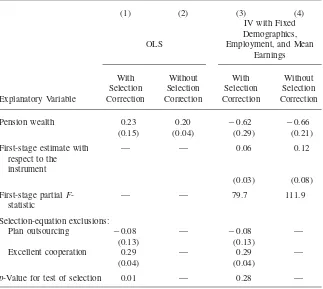
Table 2
Ordinary Least Squares (OLS) and Instrumental-Variable (IV) Estimates of the Pension Crowd-Out of Nonpension Wealth with and without Selection Correction, Standard Errors in Parentheses
Pension wealth 0.23 0.20 ⳮ0.62 ⳮ0.66
(0.15) (0.04) (0.29) (0.21)
Excellent cooperation 0.29 — 0.29 —
(0.04) (0.04)
p-Value for test of selection 0.01 — 0.28 —
Note: Each cell of the first row of the table represents a crowd-out estimate from a different selection-corrected estimation based on the subsample of 2,728 observations discussed in the text. Block-bootstrapped (by plan) standard errors based on 331 replications are shown in parentheses. All specifications include the present-value earnings measures described in the text and a baseline set of controls for the race (white), marital status (married, widowed, divorced), gender (female-headed household), any resident children, the number of resident children, education (high school, some college, college graduate), a quartic in age of the head and spouse, respectively, and interactions of the age-quartic with education and current-year earnings, plus dummy variables for union, firm-size category, and region.
and Engelhardt, Cunningham, and Kumar (2007).7One reason for measurement error in self-reported pensions in the HRS is that respondents may report their pension plan type incorrectly. For instance, a worker who really has a DC plan in which the employer’s contribution is a percentage of pay that differs with age may report
having a “formula-based” plan, which in the HRS taxonomy means a DB plan. As discussed in Section II, because each plan type has a specific sequence of questions in the survey, this would lead the respondent down the wrong path (in this case, the DB path), confronted by a set of questions inappropriate for their true plan type. This incorrect routing leads to substantial measurement error in reported plan char-acteristics that then translates into error in the calculation of pension-wealth mea-sures.
Another problem is that even if individuals correctly identify their plan type and have a good sense of the benefits their plan will eventually convey, they may have difficulty in articulating well complex plan characteristics quickly in an interview setting, such as complicated DB formulas based on salary, age, years of service, early and normal retirement dates.8 This may lead to “don’t know” responses or refusals. Indeed, the respondent-reported data may contain many missing values, which must be imputed by the researcher in order to arrive at pension wealth num-bers. Specifically, Venti and Wise (2001) reported almost 40 percent of HRS house-holds had to have had at least one piece of information imputed in order to construct their measure of self-reported pension wealth. Such imputations can result in addi-tional measurement error. Overall, documented problems in measurement have led the HRS to significantly revise and refine the pension sequence in more recent waves of the survey (Gustman, Steinmeier, and Tabatabai 2009).
In addition to these, for many pension plans, demographics, employment char-acteristics, and career earnings map into benefits in a nonlinear manner. However, most previous empirical analyses only include linear effects for these factors. If these factors also independently affect nonpension wealth accumulation nonlinearly, then previous estimates of pension crowd-out will suffer from omitted-variable bias. Fi-nally, the presence of unobserved heterogeneity would bias OLS estimates.
We attempt to circumvent these problems by constructing an instrument for self-reported pension wealth,P, in Equation 1. The instrument must be correlated with observed pension wealth, but uncorrelated with the measurement error, nonlineari-ties, and heterogeneity.
Our instrument has two components: the first component is for employer-provided pension wealth; the second component is for Social Security wealth. In the first component, for each individual in pension-covered employment on their current job, we use their actual SPD, which describes in detail all plan rules and features, in-cluding eligibility, employer contributions, benefit formulas, vesting, etc., along with information on sex, age, year of birth, earnings histories, and years of service, and pension-benefit calculators—the HRS Pension Estimation Program for DB plans, described in Curtin, Lamkin, Peticolas, and Steinmeier (1998), and the HRS DC/ 401(k) Calculatorfor DC plans, developed by Engelhardt, Cunningham, and Kumar (2007)—to construct a measure of pension wealth based on matched information.
Engelhardt and Kumar 215
A potential concern in constructing the instrument is that when the present value of pension entitlements are modeled as a function ofindividualpay, age, years of service, and survival probabilities, the instrument may be correlated with nonlinear-ities and unobserved heterogeneity and, hence, invalid. To address this, we con-structed the present values using a fixed profile of employment and demographic characteristics, corresponding (roughly) to sample mean values: year of birth (1936), hire date (1971), quit date (2001), and survival probabilities (life-table values for the birth cohort 1936). For earnings, we use the sample mean earnings (that is, unconditional mean earnings) for each year from 1951–91 taken from the adminis-trative earnings histories, so that the pension-values calculation is done for a fixed earnings profile, identical for all in our sample. Therefore, the earnings used to form the present value of pension entitlements are not based on actual individual infor-mation. For those without pension coverage on the current job, they are assigned a zero for this component of the instrument.
For the second component, we use the Social Security calculator developed by Coile and Gruber (2000) and the same inputs—fixed data on sex, age, year of birth, and years of covered work, and the sample mean earnings histories—to do a similar calculation for the present value of Social Security entitlements as we did for em-ployer-provided pensions. The SPD-based emem-ployer-provided pension and Social Security wealth components are summed to yield the instrument, which we denote as .Z
There are two sources of variation in this instrument. First, there is variation across individuals in pension coverage. Second, there is variation across pension plans in generosity.
There are two key identifying assumptions for this instrument to be valid. First, any error in the SPD-based pension wealth is uncorrelated with measurement error in the self-reported pension wealth. Second, differences across workers in pension generosity, as embodied in the instrument, are as good as random, conditional on lifetime earnings, the proxies for future earnings, demographics, and employment characteristics, that is,Cov(Z,uY,x,)⳱0. In particular, there is no sorting of work-ers to firms that offer pensions based on an unobserved taste for saving subsumed in . This is identical to what has been assumed in the previous literature on pensionsu (Gale 1998; Hubbard 1986) and the more narrowly focused literature on the impact of 401(k)s on saving (Chernozhukov and Hansen 2004; Poterba, Venti, and Wise 1995, 1996), in which 401(k) eligibility has been assumed to be conditionally ran-dom. We assess the potential impact of sorting in our robustness checks in Section V.
D. Baseline IV Estimation Results
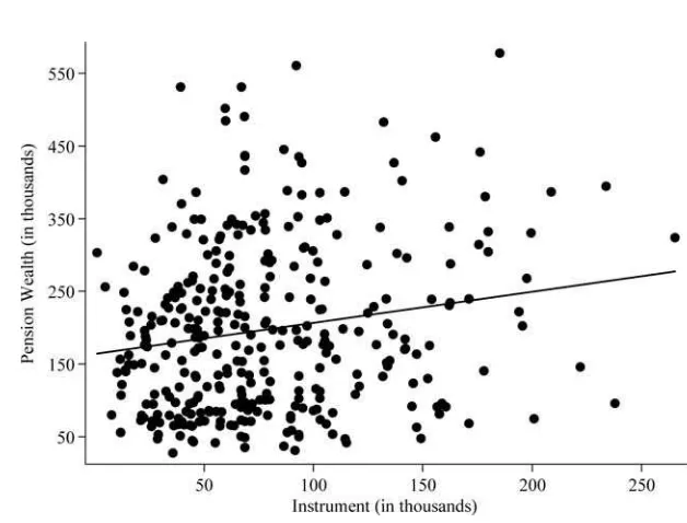
Using the cell-level data underlying the first figure, Figure 2 plots the value of P versus the instrument, . This illustrates the first-stage relationship, which is stronglyZ positive. Figure 3 plots the value of nonpension wealth versus the instrument. This illustrates the reduced-form relationship, which is negative.
block-Figure 2
Pension Wealth and the Instrument
Note: This figure shows a scatter plot of cell mean pension wealth versus the instrument, for cells defined by age, education, race, and marital status. It depicts the first-stage relationship.
bootstrapped (by plan) based on 331 replications, the Andrews-Buchinsky optimal number. The selection equation was reestimated for each bootstrap sample. We fol-low Wooldridge (2002) and include the exclusions from the selection equation in the instrument set; the associated partial F-statistic on the instrument set from the first-stage model is shown in the third row of the table.
In contrast to the OLS result in Column 1, the IV estimate is negative, ⳮ0.62, and statistically significantly different than zero, but not different than negative one, full crowd-out. The IV estimate suggests that an additional dollar of pension wealth reduces household nonpension wealth by 62 cents. Furthermore, a comparison of the OLS and IV estimates suggests that the former is severely upward biased, with ap-value for the Hausman test of 0.02. The IV estimate without selection correction (Column 4) is similar, showing crowd-out of 66 cents.
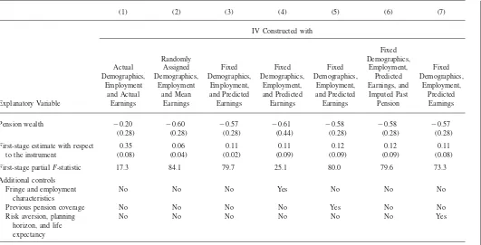
IV. Extensions and Robustness Checks
Engelhardt and Kumar 217
Figure 3
Nonpension Wealth and the Instrument
Note: This figure shows a scatter plot of cell mean nonpension wealth versus the instrument, for cells defined by age, education, race, and marital status. It depicts the reduced-form relationship.
assumption that error in the SPD-based measure of pension wealth is uncorrelated with the error in self-reported pension wealth and fixing characteristics helps to strip away the impact of unobserved heterogeneity, a comparison between the OLS and the IV estimate based on this new instrument should isolate the bias to OLS from measurement error. The IV estimate in Column 1 isⳮ0.20, with a standard error of 0.28. Thus, approximately one-half of the difference in the OLS and IV estimates in Table 2 is due to measurement error in self-reported pension wealth, with the remainder due to the nonlinearities and unmeasured heterogeneity.
We explore robustness in the remaining columns of Table 3. In Column 2, we recalculate our instrument using the worker’s own SPD, but randomly assigned dem-ographic and employment characteristics and mean earnings. The assignment was done such that, when aggregated across individuals, the assigned probabilities of having a given profile of demographics match the probability in the overall sample. The crowd-out estimate in Column 2 is 60 cents, similar to that with the basic instrument.
im-The
Journal
of
Human
Resources
Additional Instrumental-Variable (IV) Estimates of the Pension Crowd-Out of Nonpension Wealth, Standard Errors in Parentheses
(1) (2) (3) (4) (5) (6) (7)
(0.28) (0.28) (0.28) (0.44) (0.28) (0.28) (0.28)
First-stage estimate with respect to the instrument
0.35 0.06 0.11 0.11 0.12 0.12 0.11
(0.08) (0.04) (0.02) (0.09) (0.09) (0.09) (0.08)
First-stage partialF-statistic 17.3 84.1 79.7 25.1 80.0 79.6 73.3
Additional controls Fringe and employment
characteristics
No No No Yes No No No
Previous pension coverage No No No No Yes No No
Risk aversion, planning horizon, and life expectancy
No No No No No No Yes
Engelhardt and Kumar 219
posed from below by zero earnings from labor force nonparticipation and from above by the FICA taxable maximum for the following specification:
G H
OwnEduc g h White
ln (y )⳱ Ⳮ D Ⳮ Age Ⳮ D ⳭmⳭ .
(2) it 1t
兺
2gt i兺
4ht it 5t i i itg⳱1 h⳱1
The dependent variable, ln(y), is the natural log of real covered earnings (nominal covered-earnings from the database deflated into 1992 dollars by the all-items Con-sumer Price Index, or CPI). The earnings equation employs a flexible functional form that allows for (reading the terms on the right-hand side of the equation from right to left in order) calendar-year effects; time-varying returns to the respondent’s education, measured by educational attainment group,g(high school graduate, some college, college graduate, graduate degree); time-varying quartic age-earnings pro-files (H⳱4); and time-varying white-nonwhite earnings gaps. In addition, the spec-ification includes a vector of explanatory variables,m, which include a large set of time-invariant differences in earnings that are interpreted as part of the individual’s human capital endowment: an indicator for whether U.S. born; sets of indicators for mother’s and father’s education, respectively, measured by educational attainment group (high school graduate, some college, college graduate, education not reported); own Census region of birth; and interactions of race, education, and region of birth. The parameters in (2) were estimated separately by sex using Social Security earnings data from 1951 to 1991 for all HRS individuals with matched earnings histories. These estimates, with actual values of education, age, and the variables in for those individuals in the analysis sample, were used to make the predicted log m
earnings for each year from 1951 to 1991 and then were exponentiated to form an earnings history (in levels) for each individual in the analysis sample. This predicted earnings history, along with the fixed demographic and employment characteristics, was then used as an input into the pension calculators described above to generate the instrument.
Now, there are three sources of variation in this instrument based on predicted earnings. First, there is variation across individuals in pension coverage. Second, there is variation across plans in generosity. Third, there is variation within plans across workers with different predicted earnings, which occurs because some plans have benefit schedules that are nonlinear in pay, and there are some plans in the SPD database that are large enough to have multiple workers in the HRS sample.9 The associated IV estimate ofis shown in Column 3 of Table 3. The IV estimate is ⳮ0.57and statistically significantly different than zero. It suggests that an addi-tional dollar of pension wealth reduces household nonpension wealth by 57 cents. Once demographic and employment characteristics are fixed as inputs to the pension
calculators, the similarity in the estimate in Column 3 here and that in Column 3 of Table 2 (ⳮ0.57vs. ⳮ0.62) suggests that additional nonlinearities associated with the observed determinants of earnings used in the earnings Equation 2 are not gen-erating substantial omitted-variable bias in the crowd-out estimates.
In Column 4 of Table 3, we perform another robustness check by adding two large sets of controls. First, controls for nonpension fringe benefits on the current job: dummy variables for whether the firm offered long-term disability and group term life insurance, respectively, as well as the number of health insurance plans, number of retiree health insurance plans, weeks paid vacation, and days of sick pay. Second, other controls for employment characteristics: dummy variables for both the worker and spouse for whether the firm offered a retirement seminar, discussed retirement with co-workers, whether responsible for the pay and promotion of others, the number of supervisees, and a full set of occupation dummies. Although some-what less precise, the results in Column 4 suggest crowd-out of a similar magnitude, 61 cents. In fact, the p-value for the test of the null hypothesis that crowd-out,, is equal across Columns 3 and 4 is 0.70.
V. Additional Robustness Checks for Sorting
Because the instruments used thus far are based on the worker’s actual SPD, a key threat to a causal interpretation from the crowd-out estimates is the potential for endogenous sorting. For example, workers with a high taste for saving may sort themselves to firms that offer pensions (Allen, Clark, and Mc-Dermed 1993; Curme and Even 1995; Ippolito 1997; Even and McPherson 1997). If so, then the crowd-out estimates thus far in Tables 2 and 3 are biased toward zero, indicating too little crowd-out. Sorting in this direction is what typically has been discussed in the literature on the saving impact of IRAs, 401(k)s, and pen-sions—namely, “savers” save more in all forms, including pensions. Alternatively, if workers with commitment problems sort to pension-covered jobs as a way to force saving, then the basic crowd-out estimates are biased away from zero, indicating too much crowd-out. Firms also may have adopted pensions in response to employee interest, especially small firms. In a survey by Buck Consultants (1989), employee interest was cited as a reason for 401(k) adoption by 63.5 percent of firms. Finally, Ippolito (1997) has argued that firms may have used 401(k)s, and employer match-ing, in particular, to direct additional compensation to workers with a low rate of time preference as part of an optimal employee-retention policy. In any of these cases, sorting that is correlated with the instrument would render our IV crowd-out estimates invalid.
Unfortunately, because the HRS first interviews individuals in their mid 50’s and has sparse retrospective information (including no retrospective information on wealth), it is not an ideal data source to explore the impact of sorting over the career. Consequently, we assess whether sorting confounds our IV estimates using a series of approaches that best exploit the HRS data available, but none of which are iron-clad.
Engelhardt and Kumar 221
seek pension-covered jobs, then past coverage should be correlated with current coverage for these workers, and because current coverage is an important source of variation in our instrument, then past coverage might confound our IV estimates.
We assess the impact of this in two ways. First, we utilize the retrospective in-formation gathered in the 1992 survey on job histories and prior pension coverage and present in Column 5 of Table 3 the crowd-out estimates from a modified version of Equation 1,
PrevJob1Cov PrevJob23Cov
ˆ
W⳱PⳭYiⳭ␣xⳭ␥ⳭⳭ D ⳭD Ⳮu
(3) i i i i i 1 i 2 i i
in which indicators for coverage on the most recent previous job (“previous job 1”), , and the second and third previous jobs (“previous jobs 2 or 3”),
PrevJob1Cov
D
, respectively, have been added. If workers sort, past coverage can be
PrevJobs23Cov
D
thought of as a proxy for the omitted variable that is the unobserved taste for saving. In particular, if past coverage both predicts current coverage and is correlated with the unobservable, then the IV estimate of should change substantially from that in Column 3 of Table 3, reflecting the omitted-variable bias from sorting. The es-timation results for Equation 3 are shown in Column 5 of Table 3. The IV estimate,
, is almost identical to that in Column 3.10 ˆ
⳱ⳮ0.58
Second, we remade the instrument in Column 3 of Table 3 by imputing past pension benefits at the one-digit industry level for those with pension coverage but no matched SPD on the past job. The IV estimates based on this alternative instru-ment are shown in Column 6 of the table and are very similar, showing about 58 cents crowd-out.
Next, a number of previous studies have suggested that sorting is done on the basis of risk aversion, discount rate, and life expectancy. For example, workers with low discount rates and long life expectancies should be particularly attracted to firms offering deferred compensation in the form of pensions. Thus, in Column 7 of Table 3, we added to our specification from Column 3 variables that proxy for these factors. Our measure of risk aversion is based on Barsky et al. (1998), and our proxy for the discount rate is a set of dummy variables for the household’s reported financial planning horizon, based on the following HRS question:
“In deciding how much of their (family) income to spend or save, people are likely to think about different financial planning periods. In planning your (fam-ily’s) saving and spending, which of the time periods listed is most important to you?”
where the possible answers were
“next few months, next year, next few years, next five to ten years, longer than ten years.”
Finally, we include two measures of life expectancy based on the following HRS question:
“Using any number from zero to ten, where 0 equals absolutely no chance and ten equals absolutely certain, what do you think are the chances that you will live to be 75 or more?”
(and an isomorphic question for the chances of living to be 85 or more). The as-sociated IV estimate in Column 7 is 57 cents, in the same general range as the other estimates.
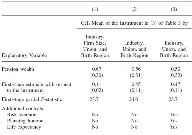
Finally, Column 1 of Table 4 presents the crowd-out estimates for the specification in Column 3 of Table 3 that use an instrument based not on the worker’s actual SPD, but based on the mean instrument for similar workers. Specifically, we divided the sample into cells based on industry, firm size, union, and region of birth and then collapsed the instrument from our preferred specification in Column 3 of Table 3 to yield a leave-one-out cell-mean instrument. We then use this as our instrumental variable. This cell-mean instrument should be less susceptible to any concerns about sorting, because for any worker, the cell-mean instrument does not depend on the actual SPD, but on the average of others with similar characteristics in the sample. The IV estimates in Column 1 of Table 4 indicate that an additional dollar of pension wealth reduces household nonpension wealth by 67 cents. This is qualitatively simi-lar to what was found when the instrument was based on the actual SPD.
Column 2 of Table 4 repeats this exercise, but now collapsing only by industry, union, and birth region, to account for potential sorting across firm size. The IV crowd-out now is 56 cents. The specification in Column 3 adds controls for risk aversion, planning horizon, and life expectancy, and the results are similar.
In summary, while each of these approaches has strengths and weaknesses in evaluating the potential impact of sorting, the IV estimates are very similar across approaches and suggest substantial crowd-out, in the 53–67 cent range. The weight of the evidence suggests that sorting is not confounding our IV crowd-out estimates.
VI. Impact Across the Wealth Distribution
There are two key drawbacks to the crowd-out estimates thus far. First, they are based on mean-regression estimators, which are sensitive to skewness in the distribution of wealth. Second, the response of household wealth accumulation to pensions is summarized in a single number. There is no allowance for differential response of nonpension wealth to pension wealth across the wealth distribution (Bi-tler, Gelbach, and Hoynes 2006).
Engelhardt and Kumar 223
Table 4
Additional Instrumental-Variable (IV) Estimates of the Pension Crowd-Out of Nonpension Wealth, Standard Errors in Parentheses
(1) (2) (3)
Cell Mean of the Instrument in (3) of Table 3 by
Explanatory Variable First-stage partialF-statistic 23.7 24.0 23.7 Additional controls
Risk aversion No No Yes
Planning horizon No No Yes
Life expectancy No No Yes
Note: Each cell of the first row of the table represents a crowd-out estimate from a different selection-corrected estimation based on the subsample of 2,728 observations discussed in the text. Block-bootstrapped (by cell) standard errors based on 331 replications are shown in parentheses. All specifications include the present-value earnings measures described in the text and a baseline set of controls for the race (white), marital status (married, widowed, divorced), gender (female-headed household), any resident children, the number of resident children, education (high school, some college, college graduate), a quartic in age of the head and spouse, respectively, and interactions of the age-quartic with education and current-year earnings, plus dummy variables for union, firm-size category, and region.
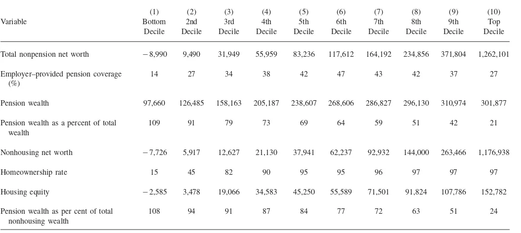
and Stafford 1998). In particular, Americans in the lower part of the wealth distri-bution have very little wealth beyond pensions and owner-occupied housing. One implication of this is that we might expect a marginal increase in pension wealth to have a very small crowd-out effect in the lower part of the wealth distribution simply because these households have very few other assets to crowd-out. Indeed, only in the upper portions of the wealth distribution is nonpension wealth likely large enough for substantial crowd-out to occur.
The
Journal
of
Human
Resources
Table 5
Sample Means for Selected Wealth and Ownership Measures by Decile of the Total Nonpension Net Worth Distribution
(1) (2) (3) (4) (5) (6) (7) (8) (9) (10)
Variable Bottom
Decile
2nd Decile
3rd Decile
4th Decile
5th Decile
6th Decile
7th Decile
8th Decile
9th Decile
Top Decile
Total nonpension net worth ⳮ8,990 9,490 31,949 55,959 83,236 117,612 164,192 234,856 371,804 1,262,101
Employer–provided pension coverage (%)
14 27 34 38 42 47 43 42 37 27
Pension wealth 97,660 126,485 158,163 205,187 238,607 268,606 286,827 296,130 310,974 301,877
Pension wealth as a percent of total wealth
109 91 79 73 69 64 59 51 42 21
Nonhousing net worth ⳮ7,726 5,917 12,627 21,130 37,941 62,237 92,932 144,000 263,466 1,176,938
Homeownership rate 15 45 82 90 95 95 96 97 97 97
Housing equity ⳮ2,585 3,478 19,066 34,583 45,250 55,589 71,501 91,824 107,786 152,782
Pension wealth as per cent of total nonhousing wealth
108 94 91 87 84 77 72 63 51 24
Engelhardt and Kumar 225
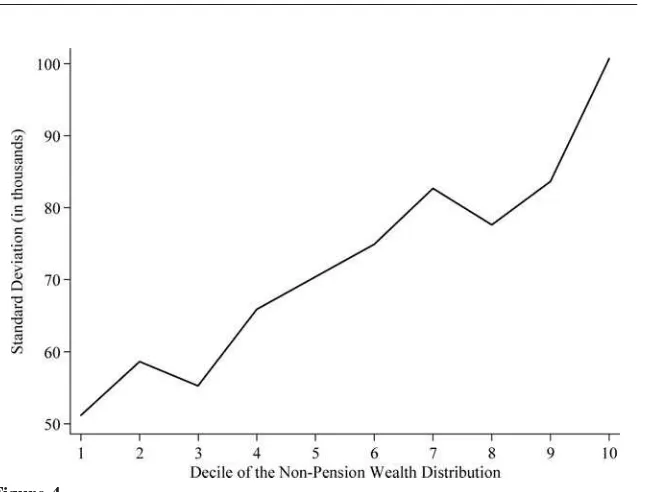
Figure 4
Standard Deviation of the Instrument by Wealth Decile
Note: This figure shows a line graph of the standard deviation of the instrument for selected deciles of the wealth distribution and illustrates there is substantial variation in the instrument by wealth level.
fifth quantile (from the tenth through the 90th) of the distribution of nonpension net worth.11
In Figure 4, we illustrate the independent variation in the instrument across the nonpension wealth distribution. Namely, we plot for each decile of the nonpension wealth distribution the standard deviation of the residuals from the auxiliary regres-sion of the instrument on all of the exogenous regressors in the specification. There is variation in the instrument at all parts of the distribution, but as one moves higher in the wealth distribution, the independent variation in the instrument rises.
The OQR and the IVQR estimates and 90 percent nonparametric bootstrapped confidence intervals are plotted in Figures 5 and 6, respectively. All estimates in the figures are corrected for potential nonrandom sample selection bias using the two-step approach of Newey (1999). In particular, in the first-two-step we estimated the selection equation semi-parametrically, along the lines of Das, Newey, and Vella (2003), using the two exclusions already outlined, and then in place of ˆ in (1)
11. Technically, this estimator requires that the disturbance term,u, contain a ranking variable, call itv
Figure 5
Ordinary Quantile Regression Estimates for Crowd-Out with 90% Confidence Intervals
Note: The solid line in the figure shows the ordinary quantile regression crowd-out estimates for selected quantiles of the nonpension wealth distribution. The dashed lines show the boundaries of the associated 90 percent confidence intervals.
included a quartic of the propensity score from the selection equation in the crowd-out equation estimated by OQR and IVQR, respectively. Newey (1999) proves the consistency of this estimator. Both the OQR and IVQR results were robust to var-iations in the order of the selection-correction polynomial beyond a quartic. When bootstrapping the confidence intervals shown in Figures 5 and 6, the selection equa-tion was re-estimated with each of the 331 bootstrap replicaequa-tions.
Across quantiles, the OQR estimates of the pension crowd-out in Figure 5 are analogous to the OLS estimates in Table 2 in that the estimated offsets are positive at all points of the wealth distribution, indicating that pensions crowd in saving. Although less precise, the IVQR estimates in Figure 6 indicate, in contrast, consid-erable heterogeneity in crowd-out.12At lower wealth quantiles, the offsets actually are positive, and around the median are not statistically different than zero. These results are not inconsistent with our expectation of little crowd-out for lower-wealth households and may suggest that households in the lower portions of the wealth
Engelhardt and Kumar 227
Figure 6
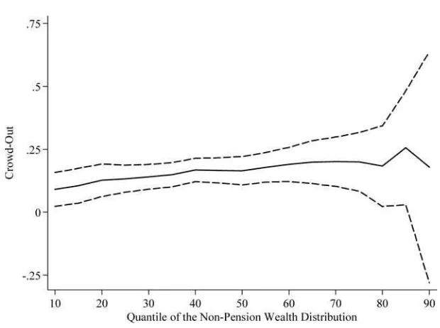
Instrumental Variable Quantile Regression Estimates for Crowd-Out with 90% Confidence Intervals
Note: The solid line in the figure shows the instrumental variable quantile regression crowd-out estimates for selected quantiles of the nonpension wealth distribution. The dashed lines show the boundaries of the associated 90 percent confidence intervals.
distribution may save more as they come in contact with pensions, an important part of the financial system. However, for 80th-90th percentiles, the crowd-out is 30–50 cents. The crowd-out at the 95th percentile (not shown) is ⳮ75 cents, but with a very large confidence interval (0,ⳮ1.5).
To further examine the extent to which the wealth response to pensions differs across households, we follow Gale (1998) and split the sample along three dimen-sions, median net worth, median income, and college education.13 The associated estimation results, which are briefly summarized in Table 6, reinforce the quantile regression results: there is substantial variation across households in the pension offset to saving, with the bulk of crowd-out occurring in the upper levels of the income/wealth distribution.
The
Journal
of
Human
Resources
Table 6
Instrumental-Variable (IV) Crowd-Out Estimates for Selected Sub-Samples Based on Economic Status, Standard Errors in Parentheses
(1) (2) (3) (4) (5) (6)
Nonpension Net Worth Income Education
Explanatory Variable
Above the Median
Below the Median
Above the Median
Below the Median
College Graduate or
Higher
Less than College Graduate
Pension wealth ⳮ0.98 0.16 ⳮ1.14 0.01 ⳮ0.70 ⳮ0.45 (0.41) (0.04) (0.33) (0.35) (0.15) (0.27)
p-value for test of equal crowd-out 0.01 0.12 0.56
Engelhardt and Kumar 229
VII. Conclusion
Our results suggest significant crowd-out, ranging from 53 to 67 cents at the mean. Compared to what has been found relatively recently in the previous literature, these estimates are, broadly speaking, similar in magnitude to those by Gale (1998), who found that pensions crowd-out total net worth by 40–83 cents per dollar of pension wealth using median and robust regression estimators on a sample of households of all ages from the 1983 Survey of Consumer Finances, and Khitatrakun, Kitamura, and Scholz (2001) in the HRS.14
Instrumenting matters a great deal, suggesting that unobserved heterogeneity, non-linearities, and measurement error impart substantial bias. The OLS results suggest crowd-in, whereas the IV estimates flip sign and are precise enough to show sub-stantial crowd-out of nonpension wealth. Similarly, the OQR results uniformly sug-gest crowd-in, but for the upper quantiles of the wealth distribution, the IVQR estimates flip sign and indicate crowd-out.15 Finally, there was substantial hetero-geneity in the estimated crowd-out across the wealth distribution, with zero offsets at or below the median, and the bulk of the mean effect concentrated in the upper quantiles.16
Overall, our results suggest that policies that raise pension wealth also will raise household wealth and will improve retirement-income adequacy. However, the im-pact will be far less for higher-wealth households, for whom crowd-out is the most important. In contrast, policies targeted to increase pension wealth for lower-wealth households will raise overall household wealth accumulation essentially dollar-for-dollar.
There are two important caveats to this analysis. This analysis says little directly about one of the most important recent trends in pension provision, the impact of automatic enrollment in 401(k) plans on household saving, because none of the 401(k) plans included in this study (circa 1992) had automatic enrollment.17Given the rapid adoption of automatic enrollment, assessing the impact of such default policies on wealth accumulation is a first-order question. To the extent that automatic enrollment increases participation among households in the lower part of the wealth distribution (Madrian and Shea 2001), the results of this analysis would seem to suggest that increased saving through automatic enrollment would increase
house-14. Although this paper focuses on crowd-out in the United States, the results herein are, broadly speaking, also consistent with the two best recent papers in this area by Attanasio and Rohwedder (2003) and Attanasio and Brugiavini (2003), who found substantial substitutability between pensions and household saving in the United Kingdom and Italy, respectively.
15. Gale (1998) found substantial offset at the median without instrumenting. How much this is due to using an SCF sample with a broader age range, and how much of this is due to the dramatic changes in the pension landscape from 1983, when the SCF data were gathered, to 1992, when the HRS data were gathered, are open questions (Gale and Milano, 1998).
16. Gale (1998) also documented substantial heterogeneity in response, a theme that emerged in this analysis and many other studies as well, but using sample-splitting techniques that differ from the IVQR approach used here. The IVQR results in this paper are consistent with those of Chernozhukov and Hansen (2004), who found, at higher quantiles, an increasing degree of substitution of 401(k) for other assets using data from the Survey of Program Participation (SIPP).
hold wealth and not be undone by a reduction in nonpension wealth, but that is an open question. In addition, this analysis focused on older households from the HRS, and these results may not fully characterize the saving response of younger workers to changes in pension benefits.
References
Allen, Steven G., Robert L. Clark, and Ann A. McDermed. 1993. “Pensions, Bonding, and Lifetime Jobs.”Journal of Human Resources28(3):463–81.
Andrews, Donald W. K., and Moshe Buchinsky. 2000. “A Three-Step Method for Choosing the Number of Bootstrap Repetitions.”Econometrica68(1):23–51.
Attanasio, Orazio P., and Agar Brugiavini. 2003. “Social Security and Households’ Saving.” Quarterly Journal of Economics118(3):1075–1119.
Attanasio, Orazio P., and Susann Rohwedder. 2003. “Pension Wealth and Household Saving: Evidence from Pension Reforms in the United Kingdom.”American Economic Review 93(5):1499–1521.
Avery, Robert B., Gregory E. Elliehausen, and Thomas A. Gustafson. 1986. “Pensions and Social Security in Household Portfolios: Evidence from the 1983 Survey of Consumer Finances.” InSavings and Capital Formation: The Policy Options, ed. F. Gerard Adams and S. M. Wachter, 127–60. Lexington, Mass.: Lexington Books.
Barsky, Robert B., F. Thomas Juster, Miles S. Kimball, and Matthew D. Shapiro. 1998. “Preference Parameters and Behavioral Heterogeneity: An Experimental Approach in the Health and Retirement Study.”Quarterly Journal of Economics112(2):537–80. Berger, M., D. Black, and F. Scott. 2000. “Bounding Parameter Estimates with
Non-Classical Measurement Error.”Journal of the American Statistical Association 95(451):739–48.
Bitler, Marianne P., Jonah P. Gelbach, and Hilary W. Hoynes. 2006. “What Mean Impacts Miss: Distributional Effects of Welfare Reform Experiments.”American Economic Review 96(4):988–1012.
Blinder, Alan S., Roger H. Gordon, and Donald E. Wise. 1980. “Reconsidering the Work Disincentive Effects of Social Security.”National Tax Journal33(4):431–42.
Browning, Martin, and Annamaria Lusardi. 1996. “Household Saving: Micro Theories and Micro Facts.”Journal of Economic Literature34(4):1797–1855.
Buck Consultants, Inc. 1989.Current 401(k) Plan Practices: A Survey Report. Secaucus, NJ: Buck Consultants, Inc.
Cagan, Phillip. 1965. “The Effect of Pension Plans on Aggregate Saving: Evidence from a Sample Survey.” National Bureau of Economic Research Occasional Paper No. 95. Chernozhukov, Viktor, and Christian Hansen. 2004. “The Effect of 401(k) Participation on
the Wealth Distribution: An Instrumental Quantile Regression Analysis.”Review of Economics and Statistics86(3):735–51.
Chernozhukov, Viktor, and Christian Hansen. 2005. “An IV Model of Quantile Treatment Effects.”Econometrica73(1):245–61.
Choi, James J., David Laibson, and Brigitte C. Madrian. 2004. “Plan Design and 401(k) Savings Outcomes.”National Tax Journal57(2):275–98.
Choi, James J., David Laibson, Brigitte C. Madrian, and Andrew Metrick. 2002. “Defined Contribution Pensions: Plan Rules, Participant Decisions, and the Path of Least Resistance.” InTax Policy and the Economy, Vol. 16, ed. J.M. Poterba, 67–114. Cambridge, MA: MIT Press.
Engelhardt and Kumar 231
———. 2004. “For Better or Worse: Default Effects and 401(k) Savings Behavior.” In Perspectives in the Economics of Aging, ed. D. A. Wise, 81–125. Chicago: University of Chicago Press.
Coile, Courtney, and Jonathan Gruber. 2000. “Social Security and Retirement.” NBER Working Paper 7830.
Cunningham, Christopher R., and Gary V. Engelhardt. 2002. “Federal Tax Policy, Employer Matching, and 401(k) Saving: Evidence from HRS W-2 Records.”National Tax Journal 55(3):617–45.
Curme, Michael A., and William E. Even. 1995. “Pension Coverage and Borrowing Constraints.”Journal of Human Resources30(4):701–12.
Curtin, Richard, Jody Lamkin, Bob Peticolas, and Thomas Steinmeier. 1998. “The Pension Calculator Program for the Health and Retirement Study (Level 2: Pre-Compiled Version).” Unpublished.
Das, Mitali, Whitney K. Newey, and Francis Vella. 2003. “Nonparametric Estimation of Sample Selection Models.”Review of Economic Studies70(1):33–63.
Diamond, Peter A., and Jerry A. Hausman. 1984. “Individual Retirement and Savings Behavior.”Journal of Public Economics23(1):81–114.
Duflo, Esther, William Gale, Jeffrey Liebman, Peter Orszag, and Emmanuel Saez. 2006. “Saving Incentives for Low- and Middle- Income Families: Evidence from a Field Experiment with H&R Block.”Quarterly Journal of Economics121(4):1311–46. Engelhardt, Gary V., Christopher R. Cunningham, and Anil Kumar. 2007. “Measuring
Pension Wealth.” InRedefining Retirement: How Will Boomers Fare?ed. O. Mitchell, B. Soldo, and B. Madrian, 211–33. Oxford: Oxford University Press.
Engelhardt, Gary V., and Anil Kumar. 2007. “Employer Matching and 401(k) Saving: Evidence from the Health and Retirement Study.”Journal of Public Economics 91(10):1920–43.
Engen, Eric M., William G. Gale, and John Karl Scholz. 1996. “The Illusory Effects of Saving Incentives on Saving.”Journal of Economic Perspectives10(4):113–37.
Even, William E., and David A. Macpherson. 1997. “Factors Influencing Participation and Contribution Levels in 401(k) Plans.” Miami University (Ohio). Unpublished.
Feldstein, Martin. 1974. “Social Security, Induced Retirement, and Aggregate Capital Accumulation.”Journal of Political Economy82(5):905–26.
———. 1996. “Social Security and Savings: New Time Series Evidence.”National Tax Journal46(2):151–64.
Feldstein, Martin, and Anthony Pellechio. 1979. “Social Security and Household Wealth Accumulation: New Microeconometric Evidence.”Review of Economics and Statistics 61(3):361–68.
Gale, William G. 1998. “The Effects of Pensions on Household Wealth: A Re-Evaluation of Theory and Evidence.”Journal of Political Economy106(4):706–23.
Gale, William G., Michael Dworksy, John Phillips, and Leslie Muller. 2007. “Effects of After-Tax Pension and Social Security Benefits on Household Wealth: Evidence from a Sample of Retirees.” Brookings Institution. Unpublished.
Gale, William G., and Joseph M. Milano. 1998. “Implications of the Shift to Defined Contribution Plans for Retirement Wealth Accumulation.” InLiving with Defined Contribution Pensions, ed. O.S. Mitchell and S.J. Schieber, 115–35. Philadelphia: University of Philadelphia Press.
Gustman, Alan L., and Thomas L. Steinmeier. 1999. “Effects of Pensions on Savings: Analysis with Data from the Health and Retirement Study.”Carnegie-Rochester Series on Public Policy50(1):271–326.
———. 2004. “What People Don’t Know About Pensions and Social Security.” InPrivate Pensions and Public Policies, ed. W. G. Gale, J. B. Shoven, and M. J. Washawsky, 57– 125. Washington, D.C.: Brookings Institution Press.
Gustman, Alan L., Thomas L. Steinmeier, and Nahid Tabatabai. 2009. “Do Workers Know About Their Pension Plan Type? Comparing Workers’ and Employers’ Pension Information.” InOvercoming the Saving Slump: How to Increase the Effectiveness of Financial Education and Saving Programs, ed. A. Lusardi, 47–81. Chicago: University of Chicago Press.
Hubbard, R. Glenn. 1986. “Pension Wealth and Individual Saving.”Journal of Money, Credit, and Banking18(2):167–78.
Hubbard, R. Glenn, and Jonathan S. Skinner. 1996. “Assessing the Effectiveness of Saving Incentives.”Journal of Economic Perspectives10(4):73–90.
Hurd, Michael D. 1989. “Mortality Risk and Bequests.”Econometrica57(4):779–813. Hurst, Erik, Ming Ching Luoh, and Frank Stafford. 1998. “The Wealth Dynamics of
American Families, 1984–94.”Brookings Papers on Economic Activity1998(1):267–337. Ippolito, Richard A. 1997.Pension Plans and Employee Performance: Evidence, Analysis,
and Policy. Chicago: University of Chicago Press.
Johnson, Richard W., Usha Sambamoorthi, and Stephen Crystal. 2000. “Pension Wealth at Midlife: Comparing Self-Reports with Provider Data.”Review of Income and Wealth 46(1):59–83.
Kane, Thomas, Cecilia Rouse, and Douglas Staiger. 1999. “Estimating the Returns to Schooling when Schooling is Misreported.” NBER Working Paper 7235.
Katona, George. 1965.Private Pensions and Individual Saving. Ann Arbor: University of Michigan, Survey Research Center, Institute for Social Research.
Khitatrakun, Surachai, Yuichi Kitamura, and John Karl Scholz. 2001. “Pensions and Wealth: New Evidence from the Health and Retirement Study.” University of Wisconsin-Madison. Unpublished.
Kotlikoff, Laurence J. 1979. “Testing the Theory of Social Security and Life-Cycle Accumulation.”American Economic Review69(3):396–410.
Leimer, Dean R., and Selig D. Lesnoy. 1982. “Social Security and Private Saving: New Time-Series Evidence.”Journal of Political Economy90(3):606–29.
Madrian, Brigitte C., and Dennis F. Shea. 2001. “The Power of Suggestion: Inertia in 401(k) Participation and Savings Behavior.”Quarterly Journal of Economics 116(4):1149–87.
Mitchell, Olivia S. 1988. “Worker Knowledge of Pension Provisions.”Journal of Labor Economics6(1):21–39.
Mitchell, Olivia S., Jan Olson, and Thomas Steinmeier. 1996. “Construction of the Earnings and Benefits File (EBF) for Use with the Health and Retirement Survey.”Institute for Social Research, University of Michigan, HRS/AHEAD Documentation Report No. DR-001.
Munnell, Alicia H. 1974.The Effect of Social Security on Personal Savings. Cambridge, Mass.: Ballinger.
Munnell, Alicia H. 1976. “Private Pensions and Saving: New Evidence.”Journal of Political Economy84(5):1013–32.
Newey, Whitney K. 1999. “Consistency of Two-Step Sample Selection Estimators Despite Misspecification of Distribution.”Economics Letters63(2):129–32.
Engelhardt and Kumar 233
———. 1996. “How Retirement Saving Programs Increase Saving.”Journal of Economic Perspectives10(4):91–112.
Rohwedder, Susann. 2003a. “Empirical Validation of HRS Pension Wealth Measures.” Rand Corporation. Unpublished.
———. 2003b. “Measuring Pension Wealth in the HRS: Employer and Self-Reports.” Rand Corporation. Unpublished.
Starr-McCluer, Martha, and Annika Sunden. 1999. “Workers’ Knowledge of Their Pension Coverage: A Reevaluation”Federal Reserve Board of Governors. Unpublished. Venti, Steven F., and David A. Wise. 2001. “Choice, Chance, and Wealth Dispersion at
Retirement.” InAging Issues in the United States and Japan, ed. S. Ogura, T. Tachibanaki, and D. Wise, 25–64. Chicago: University of Chicago Press.
Wooldridge, Jeffrey M. 2002.Econometric Analysis of Cross Section and Panel Data. Cambridge, Mass: MIT Press.
Appendix 1
Technical Appendix
The linear-in-parameters econometric specification we estimate in (1) in the text follows from the basic, frictionless continuous-time life-cycle model formulated by Gale (1998). The consumer lives from time 0, until known death in time ; retire-T ment occurs at time R. Utility is derived from consumption, C, is based on the isoelastic form,
exhibits constant relative risk aversion (CRRA), and is the coefficient of relative risk aversion. The consumer maximizes lifetime utility
T
subject to the intertemporal budget constraint
T R T
ⳮrt ⳮrt ⳮrt
B e dtⳭ E e dt⳱ C e dt ,
(A3)
冮
t冮
t冮
tR 0 0
whereEis labor-market earnings,Bis real public and private pension benefits,ris the real rate of return, and␦ is the rate of time preference.
A
r(Aⳮt) W ⳱ (EⳮC)e dt .
(A4) A
冮
t t0
The left-hand side of (A4) is the typical dependent variable in an econometric spec-ification for crowd-out. To express the right-hand side in terms of the present value of future pension entitlements, the typical explanatory variable of interest in a crowd-out equation, note that the first-order conditions from (A2)-(A3) imply
[(rⳮ␦) /]t
which can substituted back into (A5) and then (A4) to yield
A T R
is Gale’s Q, which takes into account the time the consumer has had since the introduction of the pension to adjust the lifetime consumption stream; whenx⳱0, . We note that this adjustment is not due to any inherent frictions in the Q⳱A/T
model, as Gale’s framework is based on a frictionless model, and, as Gale argues, is applicable even for incomplete offset. Because the last term on the right-hand side of (A7) can be expressed as
R A R
Equation (A10) is a convenient representation of nonpension wealth at a point in time, and is the basis for (1) in the text:
ˆ W⳱PⳭYⳭ␣xⳭ␥ⳭⳭu ,
(A11) i i i i i i i