of
ACOUSTICS
2.1 FREQUENCY AND WAVELENGTH
Frequency
A steady sound is produced by the repeated back and forth movement of an object at regular intervals. The time interval over which the motion recurs is called theperiod. For example if our hearts beat 72 times per minute, the period is the total time (60 seconds) divided by the number of beats (72), which is 0.83 seconds per beat. We can invert the period to obtain the number of complete cycles of motion in one time interval, which is called thefrequency.
f = 1
T (2.1)
where f =frequency (cycles per second or Hz) T=time period per cycle (s)
The frequency is expressed in units of cycles per second, or Hertz (Hz), in honor of the physicist Heinrich Hertz (1857–1894).
Wavelength
Among the earliest sources of musical sounds were instruments made using stretched strings. When a string is plucked it vibrates back and forth and the initial displacement travels in each direction along the string at a given velocity. The time required for the displacement to travel twice the length of the string is
T= 2 L
Figure2.1 Harmonics of a Stretched String (Pierce, 1983)
where T=time period (s)
L=length of the string (m) c=velocity of the wave (m /s)
Since the string is fixed at its end points, the only motion patterns allowed are those that have zero amplitude at the ends. This constraint (called aboundary condition) sets the frequencies of vibration that the string will sustain to a fundamental and integer multiples of this frequency, 2f,3f,4f, . . . ,calledharmonics. Figure 2.1 shows these vibration patterns.
f = c
2 L (2.3)
As the string displacement reflects from the terminations, it repeats its motion every two lengths. The distance over which the motion repeats is called the wavelength, and is given the Greek symbol lambda,λ, which for the fundamental frequency in a string is 2 L. This leads us to the general relation between the wavelength and the frequency
λ= c
f (2.4)
where λ=wavelength (m)
c=velocity of wave propagation (m /s) f =frequency (Hz)
Fundamentals
of
Acoustics
instruments, including the human voice, are given in Fig. 2.3. If a piano string is vibrating at its fundamental mode, the maximum excursion occurs at the middle of the string. When a piano key is played, the hammer does not strike precisely in the center of the string and thus it excites a large number of additional modes. These harmonics contribute to the beauty and complexity of the sound.
Frequency Spectrum
If we were to measure the strength of the sound produced by a particular note and make a plot of sound level versus frequency we would have a graph called aspectrum. When the sound has only one frequency, it is called apure toneand its spectrum consists of a single straight line whose height depends on its strength. The spectrum of a piano note, shown in Fig. 2.4, is a line at the fundamental frequency and additional lines at each harmonic frequency. For most notes the fundamental has the highest amplitude, followed by the harmonics in descending order. For piano notes in the lowest octave the second harmonic may have a higher amplitude than the fundamental if the strings are not long enough to sustain the lowest frequency.
Sources such as waterfalls produce sounds at many frequencies, rather than only a few, and yield a flat spectrum. Interestingly an impulsive sound such as a hand clap also yields a flat spectrum. This is so because in order to construct an impulsive sound, we add up a very large number of waves of higher and higher frequencies in such a way that their peaks all occur at one time. At other times they cancel each other out so we are left with just the impulse spike. Since the two forms are equivalent, a sharp impulse generates a large number of waves at different frequencies, which is a flat spectrum. A clap often is used to listen for acoustical defects in rooms.
Electronic signal generators, which produce all frequencies within a given bandwidth, are used as test sources. The most commonly encountered are the pink-noise (equal energy per octave or third octave) or white-noise (equal energy per cycle) generators.
Filters
In analyzing the spectral content of a sound we might use a meter that includes electronic filters to eliminate all signals except those of interest to us. Filters have a center frequency and a bandwidth, which determines the limits of the filter. By international agreement certain standard center frequencies and bandwidths are specified, which are set forth in Table 2.1. The most commonly used filters in architectural acoustics have octave or third-octave bandwidths. Three one-third octaves are contained in each octave, but these do not correspond to any given set of notes. Narrow bandwidth filters, 1/10 octave or even 1 Hz wide, are sometimes used in the study of vibration or the details of reverberant falloff in rooms.
2.2 SIMPLE HARMONIC MOTION
Fundamentals
of
Acoustics
Figure2.4 Frequency Spectrum of a Piano Note
Table2.1 Octave and Third-Octave Band Frequency Limits
Frequency, Hz
Octave One-third Octave
Band Lower Limit Center Upper Limit Lower Limit Center Upper Limit
Figure2.5 Vector Representation of Circular Functions
Vector Representation
Sinusoidal waveforms are components of circular motion. In Fig. 2.5 we start with a circle whose center lies at the origin, and draw a radius at some angleθ to the x (horizontal) axis. The anglethetacan be measured using any convenient fractional part of a circle. One such fraction is 1/360 of the total angle, which defines the unit called adegree. Another unit is 1/2πof the total angle. This quantity is the ratio of the radius to the circumference of a circle and defines theradian(about 57.3◦). It was one of the Holy Grails of ancient mathematics since it contains the value ofπ.
In a circle the triangle formed by the radius and its x and y components defines the trigonometric relations for the sine
y=r sin θ (2.5)
and cosine functions
x=r cos θ (2.6)
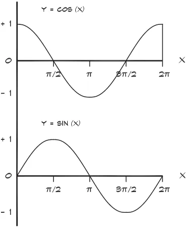
The cosine is the x-axis projection and the sine the y-axis projection of the radius vector. If we were to rotate the coordinate axes counterclockwise a quarter turn, the x axis would become the y axis. This illustrates the simple relationship between the sine and cosine functions
cos θ =sinθ +π 2
(2.7)
The Complex Plane
We can also express the radius of the circle as a vector that has x and y components by writing
r=ix+jy (2.8)
where i and j are the unit vectors along the x and y axes. If instead we define x as the displacement along the x axis and j y as the displacement along the y axis, then the vector can be written
r=x+j y (2.9)
presence or absence of the j term.
r=x+j y (2.10)
The factor j has very interesting properties. To construct the element j y, we measure a distance y along the x axis and rotate it 90◦ counterclockwise so that it ends up aligned with the y axis. Thus the act of multiplying by j, in this space, is equivalent to a 90◦rotation. Since two 90◦rotations leave the negative of the original vector
j2= −1 (2.11)
and
j= ±√−1 (2.12)
which defines j as the fundamental complex number. Traditionally, we use the positive value of j.
The Complex Exponential
The system of complex numbers, although nonintuitive at first, yields enormous benefits by simplifying the mathematics of oscillating functions. The exponential function, where the exponent is imaginary, is the critical component of this process. We can link the sinusoidal and exponential functions through their Taylor series expansions
sin θ =θ − θ
and examine the series expansion for the combination cosθ +j sinθ
cos θ +j sin θ =1+jθ− θ
This sequence is also the series expansion for the exponential function ejθ, and thus we obtain the remarkable relationship originally discovered by Leonhard Euler in 1748
Figure2.6 Rotating Vector Representation of Harmonic Motion
Using the geometry in Fig. 2.6 we see that the exponential function is another way of representing the radius vector in the complex plane. Multiplication by the exponential function generates a rotation of a vector, represented by a complex number, through the angleθ.
Radial Frequency
If the angleθ increases with time at a steady rate, as in Fig. 2.6, according to the relationship
θ =ωt+φ (2.18)
the radius vector spins around counterclockwise from some beginning angular positionφ (called theinitial phase). The rate at which it spins is the radial frequencyω, which is the angleθ divided by the time t, starting atφ = 0. Omega (ω) has units of radians per second. As the vector rotates around the circle, it passes through vertical(θ =π /2)and then back to the horizontal(θ = π ). When it is pointed straight down,θ is 3π /2 , and when it has made a full circle, thenθ is 2πor zero again.
The real part of the vector is a cosine function
x=A cos(ωt+φ) (2.19)
where x, which is the value of the function at any time t, is dependent on the amplitude A, the radial frequencyω, the time t, and the initial phase angleφ. Its values vary from−A to
+A and repeat every 2π radians.
Since there are 2π radians per complete rotation, the frequency of oscillation is
f = ω
2π (2.20)
where f =frequency (Hz)
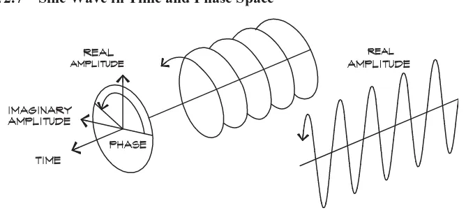
Figure2.7 Sine Wave in Time and Phase Space
It is good practice to check an equation’s units for consistency.
frequency=cycles/sec= (radians/sec)
(radians/cycle) (2.21)
Figure 2.7 shows another way of looking at the time behavior of a rotating vector. It can be thought of as an auger boring its way through phase space. If we look at the auger from the side, we see the sinusoidal trace of the passage of its real amplitude. If we look at it end on, we see the rotation of its radius vector and the circular progression of its phase angle.
Changes in Phase
If a second waveform is drawn on our graph in Fig. 2.8 immediately below the first, we can compare the two by examining their values at any particular time. If they have the same frequency, their peaks and valleys will occur at the same intervals. If, in addition, their peaks occur at the same time, they are said to be in phase, and if not, they are out of phase. A difference in phase is illustrated by a movement of one waveform relative to the other in space or time. For example, a π/2 radian (90◦) phase shift slides the second wave to the right in time, so that its zero crossing is aligned with the peak of the first wave. The second wave is then a sine function, as we found in Eq. 2.6.
2.3 SUPERPOSITION OF WAVES
Linear Superposition
Sometimes a sound is a pure sinusoidal tone, but more often it is a combination of many tones. Even the simple dial tone on a telephone is the sum of two single frequency tones, 350 and 440 Hz. Our daily acoustical environment is quite complicated, with a myriad of sounds striking our ear drums at any one time. One reason we can interpret these sounds is that they add together in a linear way without creating appreciable distortion.
Figure2.8 Two Sinusoids 90◦Out of Phase
to as a linear superposition of waves and is most useful, since it means that we can construct quite complicated periodic wave shapes by adding up contributions from many different sine and cosine functions.
Figure 2.9 shows an example of the addition of two waves having the same frequency but a different phase. The result is still a simple sinusoidal function, but the amplitude depends on the phase relationship between the two signals. If the two waves are
x1 =A1cos(ωt+φ1) (2.22)
and
x2 =A2cosωt+φ2 (2.23)
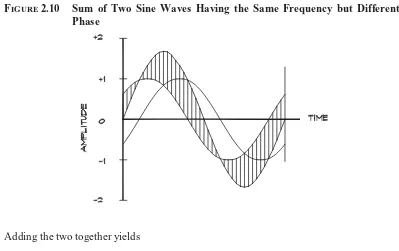
Figure2.10 Sum of Two Sine Waves Having the Same Frequency but Different
Phase
Adding the two together yields
x1 +x2 =A1cosωt+φ1+A2cosωt+φ2 (2.24)
The combination of these two waves can be written as a single wave.
x=A cos(ωt+φ) (2.25)
Figure 2.9 shows how the overall amplitude is determined. The first radius vector drawn from the origin and then a second wave is introduced. Its rotation vector is attached to the end of the first vector. If the two are in phase, the composite vector is a single straight line, and the amplitude is the arithmetic sum of A1 +A2. When there is a phase difference, and the second vector makes an angleφ2 to the horizontal, the resulting amplitude can be calculated using a bit of geometry
A=
A1cosφ1+A2cosφ22+A1sinφ1+A2sinφ22 (2.26)
and the overall phase angle for the amplitude vector A is
tanφ = A1 sinφ1+A2 sin φ2
A1 cosφ1 +A2 cosφ2 (2.27)
Thus superimposed waves combine in a purely additive way. We could have added the wave forms on a point-by-point basis (Fig. 2.10) to obtain the same results, but the mathematical result is much more general and useful.
Beats
Figure2.11 Two Complex Vectors (Feynman et al., 1989)
Figure2.12 The Sum of Two Sine Waves with Widely Differing Frequencies
If they both start at zero, then
x1 =A1cosω1 t (2.28)
and
x2 =A2cosω2 t (2.29)
The combination of these two signals is shown in Fig. 2.12. Here the two frequencies are relatively far apart and the higher frequency signal seems to ride on top of the lower frequency. When the amplitudes are the same, the sum of the two waves is1
x=2 A cos ω1−ω2
2
cos ω1+ω2
2
(2.30)
If the two frequencies are close together, a phenomenon known as beats occurs. Since one-half the difference frequency is small, it modulates the amplitude of one-half the sum frequency. Figure 2.13 shows this effect. We hear the increase and decrease in signal strength of sound, which is sometimes more annoying than a continuous sound. In practice, beats
1The following trigonometric functions were used:
Figure2.13 The Phenomenon of Beats
are encountered when two fans or pumps, nominally driven at the same rpm, are located physically close together, sometimes feeding the same duct or pipe in a building. The sound waxes and wanes in a regular pattern. If the two sources have frequencies that vary only slightly, the phenomenon can extend over periods of several minutes or more.
2.4 SOUND WAVES
Pressure Fluctuations
A sound wave is a longitudinal pressure fluctuation that moves through an elastic medium. It is called longitudinal because the particle motion is in the same direction as the wave propagation. If the displacement is at right angles to the direction of propagation, as is the case with a stretched string, the wave is called transverse. The medium can be a gas, liquid, or solid, though in our everyday experience we most frequently hear sounds transmitted through the air. Our ears drums are set into motion by these minute changes in pressure and they in turn help create the electrical impulses in the brain that are interpreted as sound. The ancient conundrum of whether a tree falling in a forest produces a sound, when no one hears it, is really only an etymological problem. A sound is produced because there is a pressure wave, but a noise, which requires a subjective judgment and thus a listener, is not.
Sound Generation
All sound is produced by the motion of a source. When a piston, such as a loudspeaker, moves into a volume of air, it produces a local area of density and pressure that is slightly higher than the average density and pressure. This new condition propagates throughout the surrounding space and can be detected by the ear or by a microphone.
When the piston displacement is very small (less than the mean free path between molecular collisions), the molecules absorb the motion without hitting other molecules or transferring energy to them and there is no sound. Likewise if the source moves very slowly, air flows gently around it, continuously equalizing the pressure, and again no sound is created (Ingard, 1994). However, if the motion of the piston is large and sufficiently rapid that there is not enough time for flow to occur, the movement forces nearby molecules together, locally compressing the air and producing a region of higher pressure. What creates sound is the motion of an object that is large enough and fast enough that it induces a localized compression of the gas.
element in the direction of propagation, which transfer energy through alternations of high pressure and low velocity with low pressure and high velocity. It is the material properties of mass and elasticity that ensure the propagation of the wave.
As a wave propagates through a medium such as air, the particles oscillate back and forth when the wave passes. We can write an equation for the functional behavior of the displacement y of a small volume of air away from its equilibrium position, caused by a wave moving along the positive x axis (to the right) at some velocity c.
y=f(x−c t) (2.31)
Implicit in this equation is the notion that the displacement, or any other property of the wave, will be the same for a given value of(x−c t). If the wave is sinusoidal then
y=A sin [k(x−c t)] (2.32)
where k is called the wave number and has units of radians per length. By comparison to Eq. 2.19 the term (k c) is equal to theradial frequencyomega.
k= 2π λ =
ω
c (2.33)
Wavelength of Sound
The wavelength of a sound wave is a particularly important measure. Much of the behavior of a sound wave relates to the wavelength, so that it becomes the scale by which we judge the physical size of objects. For example, sound will scatter (bounce) off a flat object that is several wavelengths long in a specular (mirror-like) manner. If the object is much smaller than a wavelength, the sound will simply flow around it as if it were not there. If we observe the behavior of water waves we can clearly see this behavior. Ocean waves will pass by small rocks in their path with little change, but will reflect off a long breakwater or similar barrier. Figure 2.14 shows typical values of the wavelength of sound in air at various frequencies. At 1000 Hz, which is in the middle of the speech frequency range, the wavelength is about 0.3 m (1 ft) while for the lowest note on the piano the wavelength is about 13 m (42 ft). The lowest note on a large pipe organ might be produced by a 10 m (32 ft) pipe that is half the wavelength of the note. The highest frequency audible to humans is about 20,000 Hz and has a wavelength of around half an inch. Bats, which use echolocation to find their prey, must transmit frequencies as high as 100,000 Hz to scatter off a 2 mm (0.1 in) mosquito.
Velocity of Sound
Figure2.14 Wavelength vs Frequency in Air at 20◦C (68◦F) (Harris, 1991)
Let us construct (following Halliday and Resnick, 1966), a one-dimensional tube and set a piston into motion with a short stroke that moves to the right and then stops. The compressed area will move away from the piston with a velocity c. In order to study the pulse’s behavior it is convenient to ride along with it. Then the fluid appears to be moving to the left at the sound velocity c. As the fluid stream approaches our pulse, it encounters a region of higher pressure and is decelerated to some velocity c−c. At the back (left) end of the pulse, the fluid is accelerated by the pressure differential to its original velocity, c.
If we examine the behavior of a small element (slice) of fluid such as that shown in Fig. 2.15, as it enters the compressed area, it experiences a force
F=(P+P)S−PS (2.34)
where S is the area of the tube. The length of the element just before it encountered our pulse was ct, wheret is the time that it takes for the element to pass a point. The volume of the element is c St and it has massρc St, whereρis the density of the fluid outside the pulse zone. When the fluid passes into our compressed area, it experiences a deceleration
equal to−c/t. Using Newton’s law to relate the force and the acceleration
Now the fluid that entered the compressed area had a volume V=S ct and was compressed by an amount Sct=V. The change in volume divided by the volume is
Thus, we have related the velocity of sound to the physical properties of a fluid. The right-hand side of Eq. 2.39 is a measurable quantity called thebulk modulus, B. Using this symbol the velocity of sound is
c= B
ρ (2.40)
where c=velocity of sound (m /s)
B=bulk modulus of the medium (Pa)
ρ=density of the medium(kg/m3) which for air =1.21 kg/m3
The bulk modulus can be measured or can be calculated from an equation of state, which relates the behavior of the pressure, density, and temperature in a gas. In a sound wave, changes in pressure and density happen so quickly that there is little time for heat transfer to take place. Processes thus constrained are calledadiabatic, meaning no heat flow. The appropriate form of the equation of state for air under these conditions is
P Vγ =constant (2.41)
where P=equilibrium (atmospheric) pressure (Pa) V=equilibrium volume(m3)
Under adiabatic conditions the bulk modulus isγ P, so the speed of sound is
c=
γ P/ρ0 (2.42)
Using the relationship known as Boyle’s Law (P V=μR T whereμis the number of moles of the gas and R=8.314 joules/mole◦K is the gas constant), the velocity of sound in air (which in this text is given the symbol c0) can be shown to be
c0 =20.05TC +273.2 (2.43)
where TC is the temperature in degrees centigrade. In FP (foot-pound) units the result is
c0 =49.03TF+459.7 (2.44)
where TF is the temperature in degrees Fahrenheit.
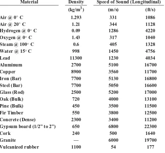
Table 2.2 shows the velocity of longitudinal waves for various materials. It turns out that the velocities in gasses are relatively close to the velocity of molecular motion due to thermal excitation. This is a reasonable result since the sound pressure changes are transmitted by the movement of molecules.
Table2.2 Speed of Sound in Various Materials (Beranek and Ver, 1992; Kinsler
and Frey, 1962)
Material Density Speed of Sound (Longitudinal)
(kg/m3) (m/s) (ft/s)
Gypsum board (1/2” to 2”) 650 6800 22300
Cork 240 500 1640
Granite — 6000 19700
Figure2.16 Shapes of Various Wave Types
Waves in Other Materials
Sound waves in gasses are only longitudinal, since a gas does not support shear or bending. Solid materials, which are bound tightly together, can support more types of wave motion than can a gas or liquid, including shear, torsion, bending, and Rayleigh waves. Figure 2.16 illustrates these various types of wave motion and Table 2.3 lists the formulas for their velocities of propagation. In a later chapter we will discuss some of the effects of flexural (bending) and shear-wave motions in solid plates. Rayleigh waves are a combination of compression and shear waves, which are formed on the surface of solids. They are most commonly encountered in earthquakes when a compression wave, produced at the center of a fault, propagates to the earth’s surface and then travels along the surface of the ground as a Rayleigh wave.
2.5 ACOUSTICAL PROPERTIES
Impedance
Table2.3 Types of Vibrational Waves and Their Velocities
Compressional
Gas Liquid Infinite Solid Solid Bar
Rectangular Bar Plate (Thickness – h) Surface of a Solid
E h2ω2
where P=equilibrium pressure (Pa)
atmospheric pressure=1.01×10⁵Pa
γ =ratio of specific heats (about 1.4 for gases) B=isentropic bulk modulus (Pa)
KB=torsional stiffness (m4) I=moment of inertia (m4)
ρ=mass density (kg / m3)
E=Young’s modulus of elasticity (N / m2)
ν=Poisson’s ratio ∼=0.3 for structural materials and∼=0.5 for rubber-like materials
T=tension (N)
ω=angular frequency (rad / s)
sound pressure to the associatedparticle velocityat a point
z= p
u (2.45)
where z=specific acoustic impedance (N s / m3) p=sound pressure (Pa)
u=acoustic particle velocity (m /s)
Figure2.17 Progression of a Pressure Pulse
of momentum so
p S=(Sρc)u (2.46)
The specific acoustic impedance of the fluid is
z= p
u =ρc (2.47)
where z=specific acoustic impedance (N s / m3or mks rayls) ρ =bulk density of the medium (kg / m3)
c=speed of sound (m / s)
The dimensions of impedance are known as rayls (in mks or cgs units) to honor John William Strutt, Baron Rayleigh. The value of the impedance frequently is used to characterize the conducting medium and is called the characteristic impedance. For air at room temperature it is about 412 mks or 41 cgs rayls.
Intensity
Another important acoustical parameter is the measure of the energy propagating through a given area during a given time. This quantity is theintensity, shown in Fig. 2.18. For a plane wave it is defined as the acoustic power passing through an area in the direction of the surface normal
I(θ )= E cos(θ )
T S =
W cos(θ )
S (2.48)
where E=energy contained in the sound wave (N m / s) W=sound power (W)
I(θ )=intensity (W / m2) passing through an area in the direction of its normal S=measurement area (m2)
T=period of the wave (s)
θ =angle between the direction of propagation and the area normal
The maximum intensity, I, is obtained when the direction of propagation coincides with the normal to the planar surface, when the angleθ =0.
I= W
S (2.49)
Plane waves are the most commonly analyzed waveform because the mathematics are simple and the form ubiquitous. A wave is considered planar when its properties do not change in the plane whose normal is the direction of propagation. Intensity is a vector quantity. Its direction is defined by the direction of the normal of the measurement area. When the normal is oriented along the direction of propagation of the sound wave, the intensity has its maximum value, which is not a vector quantity.
Sound poweris the sound energy being emitted by a source each cycle. The energy, which is the mechanical work done by a wave, is the force moving through a distance
E=p S dx (2.50)
where p is the root-mean-square acoustic pressure, and S is the area. The power, W, is the rate of energy flow so
W= p S d x
d t =p S u (2.51)
where u is the velocity of a small region of the fluid, and is called the particle velocity. It is not the thermal velocity of individual molecules but rather the velocity of a small volume of fluid caused by the passage of the sound wave. For a plane wave
I=p u (2.52)
where I=maximum acoustic intensity (W / m2)
p=root-mean-square (rms) acoustic pressure (Pa) u=acoustic rms particle velocity (m / s)
Using the definition of the specific acoustic impedance from Eq. 2.37
z= p
u =ρ c (2.53)
we can obtain for a plane wave
I= p
2
where I=maximum acoustic intensity (W / m2) p=rms acoustic pressure (Pa)
ρ =bulk density (kg / m3) c=velocity of sound (m / s)
The acoustic pressure shown in Eq. 2.44 is the root-mean-square (rms) sound pressure averaged over a cycle
which, for a sine wave, is 0.707 times the maximum value. The average acoustic pressure is zero because its value swings an equal amount above and below normal atmospheric pressure. The energy is not zero but must be obtained by averaging the square of the pressure. Interestingly, the rms pressure of the combination of random waveforms is independent of the phase relationship between the waves.
The intensity (generally taken to be the maximum intensity) is a particularly important property. It is directly measurable using a sound level meter and is audible. It is proportional to power so that when waves are combined, their intensities may be added arithmetically. The combined intensity of several sounds is the simple sum of their individual intensities. The lowest intensity that we are likely to experience is the threshold of human hearing, which is about 10−12W/m2. A normal conversation between two people might take place at about 10−6W/m2and a jet aircraft could produce 1W/m2. Thus the acoustic intensities encountered in daily life span a very large range, nearly 12 orders of magnitude. Dealing with numbers of this size is cumbersome, and has lead to the adoption of the decibel notation as a convenience.
Energy Density
In certain instances, theenergy densitycontained within a region of space is of interest. For a plane wave if a certain power passes through an area in a given time, the volume enclosing the energy is the area times the distance the sound has traveled, or c t. The energy density is the total energy contained within the volume divided by the volume
D= E
Since the range of intensities is so large, the common practice is to express values in terms oflevels. A level is basically a fraction, expressed as 10 times the logarithm of the ratio of two numbers.
Table2.4 Reference Quantities for Sound Levels (Beranek and Ver, 1992)
has a numeric value of 1, such as 1 second or 1 square meter, there must always be a reference quantity to keep the ratio dimensionless.
The logarithm of a number divided by a reference quantity is given the unit of bels, in honor of Alexander Graham Bell, the inventor of the telephone. The multiplication by 10 has become common practice, in order to achieve numbers that have a convenient size. The quantities thus obtained have units of decibels, which is one tenth of a bel. Typical levels and their reference quantities are shown in Table 2.4. Levels are denoted by a capital L with a subscript that indicates the type of level. For example, the sound power level is shown as Lw, while the sound intensity level would be LI, and the sound pressure level, Lp.
Recalling that quantities proportional to power or energy can be combined arithmeti-cally we can combine two or more levels by adding their intensities.
ITotal =I1+I2 + · · · +In (2.58)
If we are given the intensity level of a sound, expressed in decibels, then we can find its intensity by using the definition
LI =10 log I
Iref (2.59)
and the definition of the antilogarithm
I Iref =10
0.1 LI
(2.60)
When the intensities from several signals are combined the total overall intensity ratio is
ITotal
and the resultant overall level is
As an example, we can take two sounds, each producing an intensity level of 70 dB, and ask what the level would be if we combined the two sounds. The problem can be formulated as
Thus when two levels of equal value are combined the resultant level is 3 dB greater than the original level. By doing similar calculations we learn that when two widely varying levels are combined the result is nearly equal to the larger level. For example, if two levels differ by 6 dB, the combination is about 1 dB higher than the larger level. If the two differ by 10 or more the result is essentially the same as the larger level.
When there are a number of equal sources, the combination process can be simplified
LTotal =Li +10 log n (2.65)
where Li is the level produced by one source and n is the total number of like sources.
Sound Pressure Level
Thesound pressure levelis the most commonly used indicator of the acoustic wave strength. It correlates well with human perception of loudness and is measured easily with rela-tively inexpensive instrumentation. A compilation of the sound pressure levels generated by representative sources is given in Table 2.5 at the location or distance indicated.
The reference sound pressure, like that of the intensity, is set to the threshold of human hearing at about 1000 Hz for a young person. When the sound pressure is equal to the reference pressure the resultant level is 0 dB. The sound pressure level is defined as
Lp =10 log p
2
p2 ref
(2.66)
where p=root-mean-square sound pressure (Pa) pref =reference pressure, 2×10⁻⁵Pa
Since the intensity is proportional to the square of the sound pressure as shown in Eq. 2.44 the intensity level and the sound pressure level are almost equal, differing only by a small number due to the actual value versus the reference value of the air’s characteristic impedance. This fact is most useful since we both measure and hear the sound pressure, but we use the intensity to do most of our calculations.
It is relatively straightforward (Beranek and Ver, 1992) to work out the relation-ship between the sound pressure level and the sound intensity level to calculate the actual difference
Lp =LI +10 log(ρ0c0/400) (2.67)
Table2.5 Representative A-Weighted Sound Levels (Peterson and Gross, 1974)
Sound Power Level
The strength of an acoustic source is characterized by itssound power, expressed in Watts. The sound power is much like the power of a light bulb in that it is a direct characterization of the source strength. Like other acoustic quantities, the sound powers vary greatly, and a sound power levelis used to compress the range of numbers. The reference power for this level is 10−12 Watts. Sound power levels for several sources are shown in Table 2.6.
Sound power levels can be measured by using Eq. 2.49.
I= W
Table2.6 Sound Power Levels of Various Sources (Peterson and Gross, 1974)
If we divide this equation by the appropriate reference quantities
I I0 =
W/W0
S/S0
(2.69)
and take 10 log of each side we get
where S0 is equal to 1 square meter. Recalling that the sound intensity level and the sound
The small correction for the difference between the sound intensity level and the sound pressure level, when the area is in square meters, is ignored. When the area S in Eq. 2.68 is in square feet, a conversion factor is applied, which is equal to 10 log of the number of square feet in a square meter or 10.3. We then add in the small factor, which accounts for the difference between sound intensity and sound pressure level.
These formulas give us a convenient way to measure the sound power level of a source by measuring the average sound pressure level over a surface of known area that bounds the source. Perhaps the simplest example is low-frequency sound traveling down a duct or tube having a cross-sectional area, S. The sound pressure levels are measured by moving a microphone across the open area of the duct and by taking the average intensity calculated from these measurements. The overall average sound intensity level is obtained by taking 10 log of the average intensity divided by the reference intensity. By adding a correction for the area the sound power level can be calculated. This method can be used to measure the sound power level of a fan when it radiates into a duct of constant cross section. Product manufacturers provide sound power level data in octave bands, whose center frequencies range from 63 Hz (called the first band) through 8 kHz (called the eighth band). They are the starting point for most HVAC noise calculations.
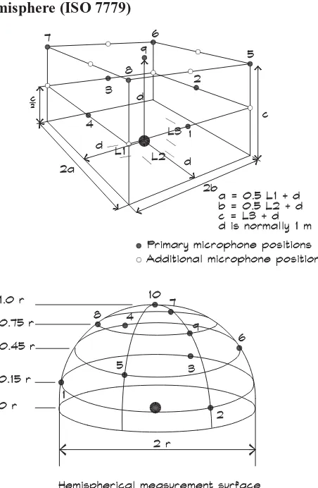
If the sound source is not bounded by a solid surface such as a duct, the area shown in Eq. 2.68 varies according to the position of the measurement. Sound power levels are determined by taking sound pressure level data at points on an imaginary surface, called themeasurement surface, surrounding the source. The most commonly used configurations are a rectangular box shape or a hemispherical-shaped surface above a hard reflecting plane. The distance between the source and the measurement surface is called themeasurement distance. For small sources the most common measurement distance is 1 meter. The box or hemisphere is divided into areas and the intensity is measured for each segment.
W=
n
i=1
Ii Si (2.72)
where W=total sound power (W)
Ii =average intensity over the i th surface (W / m2) Si =area of theith surface (m2)
n=total number of surfaces
Figure2.19 Sound Power Measurement Positions on a Parallelepiped or
Hemisphere (ISO 7779)
required if the source is long or the noise highly directional. The difference between the highest and lowest measured level must be less than the number of microphone positions. If the source is long enough that the parallelepiped has a side that is more than twice the measurement distance, the additional locations must be used.
2.7 SOURCE CHARACTERIZATION
Point Sources and Spherical Spreading
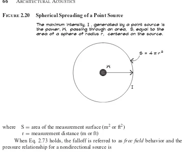
For most sources the relationship between the sound power level and the sound pressure level is determined by the increase in the area of the measurement surface as a function of distance. Sources that are small compared with the measurement distance are calledpoint sources, not because they are so physically small but because at the measurement distance their size does not influence the behavior of the falloff of the sound field. At these distances the measurement surface is a sphere with its center at the center of the source as shown in Fig. 2.20, with a surface area given by
Figure2.20 Spherical Spreading of a Point Source
where S=area of the measurement surface (m2or ft2) r=measurement distance (m or ft)
When Eq. 2.73 holds, the falloff is referred to asfree field behavior and the power-pressure relationship for a nondirectional source is
Lp =Lw+10 log
1 4π r2
+K (2.74)
where Lw =sound power level (dB re 10−12W) Lp =sound pressure level (dB re 2×10⁻⁵Pa)
r=measurement distance (m or ft) K=10 log (ρ0c0/ 400)+20 log (rref)
=0.1 for r in m, or 10.5 for r in ft (for standard conditions) rref =1 m for r in m or 3.28 ft for r in ft
The designation free field means that sound field is free from any reflections or other influences on its behavior, other than the geometry of spherical spreading of the sound energy. For a given sound power level the sound pressure level decreases 6 dB for every doubling of the measurement distance. Free-field falloff is sometimes described as 6 dB per distance doubling falloff.
Figure 2.21 shows the level versus distance behavior for a point source. If the mea-surement distance is small compared with the size of the source, where this falloff rate does not hold, the measurement position is in the region of space described as thenear field. In the near field the source size influences the power-pressure relationship. Occasionally there are nonpropagating sound fields that contribute to the sound pressure levels only in the near field.
Figure2.21 Falloff from a Point Source
to do this calculation we obtain
Lp =10 logr
2 2
r2 1
=20 logr2
r1 (2.75)
where Lp =change in sound pressure level (L1 −L2) r1 =measurement distance 1 (m or ft)
r2 =measurement distance 2 (m or ft)
Note that the change in level is positive when L1>L2, which occurs when r2>r1. As expected, the sound pressure level decreases as the distance from the source increases.
Sensitivity
Although the strength of many sources, particularly mechanical equipment, is characterized by the sound power level, in the audio industry loudspeakers are described by theirsensitivity. The sensitivity is the sound pressure level measured at a given distance (usually 1 meter) on axis in front of the loudspeaker for an electrical input power of 1 Watt. Sensitivities are measured in octave bands and are published along with the maximum power handling capacity and directivity of the device. The on-axis sound level, expected from a speaker at a given distance, can be calculated from
Lp =LS +10 log J−20 log
r rref
(2.76)
where Lp =measured on axis sound pressure level (dB)
LS =loudspeaker sensitivity (dB at 1 m for 1 W electrical input) J =electrical power applied to the loudspeaker (W)
Figure2.22 Source Directivity Shown as a Polar Plot
Directionality, Directivity, and Directivity Index
For many sources the sound pressure level at a given distance from its center is not the same in all directions. This property is calleddirectionality, and the changes in level with direction of a source are called itsdirectivity. The directivity pattern is sometimes illustrated by drawing two- or three-dimensional equal-level contours around it, such as that shown in Fig. 2.22. When these contours are plotted in two planes, a common practice in the description of loudspeakers, they are called horizontal and vertical polar patterns.
The sound power level of a source gives no specific information about the directionality of the source. In determining the sound power level, the sound pressure level is measured at each measurement position, the intensity is calculated, multiplied by the appropriate area weighting, and added to the other data. A highly directional source could have the same sound power level as an omnidirectional source but would produce a very different sound field. The way we account for the difference is by defining adirectivity index, which is the difference in decibels between the sound pressure level from an omnidirectional source and the measured sound pressure level in a given direction from the real source.
D(θ, φ)=Lp(θ, φ)−Lp (2.77)
where D(θ, φ)=directivity index (gain) for a given direction (dB) Lp(θ, φ)=sound pressure level for a given direction (dB)
Lp =sound pressure level averaged over all angles (dB) θ, φ =some specified direction
The directivity index can also be specified in terms of a directivity, which is given the symbol Q for a specific direction
D(θ, φ)=10 log Q(θ, φ) (2.78)
The directivity can be expressed in terms of the intensity in a given direction compared with the average intensity
Q(θ, φ)= I(θ, φ)
IAve (2.79)
The average intensity is given by
IAve= W
4π r2 (2.80)
and the intensity in a particular direction by
I(θ, φ)= Q(θ, φ)W
4πr2 (2.81)
When the directivity is included in the relationship between the sound power level and the sound pressure level in a given direction, the result for a point source is
Lp(θ, φ)=Lw+10 logQ(θ, φ)
4πr2 +K (2.82)
In the audio industry the Q of a loudspeaker is understood to mean the on-axis directivity, Q(0,0)=Q0.
The sound power level of a loudspeaker can be calculated from its sensitivity and its Q0 for any input power J
Lw =LS −10 log Q0
4π r2 +10 log J−K (2.83)
where LS =loudspeaker sensitivity (dB at 1 m for 1 W input) r =standard measurement distance (usually=1 m) J =input electrical power (W)
The sound pressure level emitted by the loudspeaker at a given angle can then be calculated from the sound power level
Lp =Lw+10 log Q(θ, φ)
4π r2 +K (2.84)
where Q(θ, φ)=loudspeaker directivity for a given direction Q(θ, φ)=Q0 Qrel (θ, φ)
Q0 =on - axis directivity
Qrel(θ, φ)=directivity relative to on - axis
θ, φ=latitude and longitude angles with respect to the aim point direction and the horizontal axis of the loudspeaker
Figure2.23 Falloff of a Line Source
Line Sources
Line sources are one-dimensional sound sources such as roadways, which extend over a distance that is large compared with the measurement distance. With this geometry the measurement surface is not a sphere but rather a cylinder, as illustrated in Fig. 2.23, with its axis coincident with the line source. Since the geometry is that of a cylinder the surface area (ignoring the ends) is given by the equation
S=2πrl (2.85)
where S=surface area of the cylinder (m2or ft2) r=radius of the cylinder (m or ft)
l=length of the cylinder (m or ft)
With a line source, the concept of an overall sound power level is not very useful, since all that matters is the portion of the source closest to the observer. Line sources are characterized by a sound pressure level at a given distance. From this information the sound level can be determined at any other distance.
Assume for a moment that a nondirectional line source of lengthlemits a given sound power. Then the maximum intensity at a distance r is
I= W S =
W
2πrl (2.86)
and the difference in intensity levels at two different distances can be calculated from the ratio of the two intensities
L=L1−L2 =10 log I1 Iref −
10 log I2
Iref (2.87)
So for an infinite (very long) line source the change in level with distance is given by
L=10 log I1
I2 =10 log r2
where L=change in level (dB)
L1 =sound intensity level at distance r1(dB re 10−12 W/ m2) L2 =sound intensity level at distance r2(dB re 10−12 W/ m2)
r1 =distance 1 (m or ft) r2 =distance 2 (m or ft)
If we measure the sound pressure level at a distance, r1, from an unshielded line source, we can use Eq. 2.88 to calculate the difference in level at some new distance r2. If r2 >r1then the change in level is positive—that is, sound level decreases with increasing distance from the source. The falloff rate is gentler with a line source than it is for a point source—3 dB per distance doubling.
Planar Sources
Aplanar source is a two-dimensional surface that is large compared to the measurement distance and usually, though not always, relatively flat. For purposes of this analysis a planar source is assumed to be incoherent, which is to say that there is no fixed phase relationship among the various points on its surface. From our previous analysis we know that if a surface radiates a certain acoustic power, W, and if that power is uniformly distributed over the surface, then close to the surface the intensity is given by
I= W
S (2.89)
where S is the area of the surface. We also know that if we are far enough away from the surface, it is small compared to the measurement distance, and it must behave like a point source; the intensity is given by Eq. 2.82. To model (Long, 1987) the behavior in both regions, it is convenient to imagine the planar source shown in Fig. 2.24 as a portion of a
large sphere that has a radius equal to
S Q
4π. Since the measurement distance is taken from
the surface of the plane, the distance to the center of the sphere from the measurement point
isz+
When this equation is written as a level by taking 10 log of both sides
Lp =Lw +10 log
z=measurement distance from the surface (m or ft) K=0.1 (zin m) or 10.5 (zin ft) for standard conditions