in
MECHANICAL SYSTEMS
13.1 MECHANICAL SYSTEMS
Occupied spaces need the continuous delivery of the requirements for the human habitat—air, water, power, a controlled thermal environment—and the return of the waste products back to the surroundings in the form of carbon dioxide, waste water, sewage, refuse, and heat. To carry out these functions specialized machines are included in every building. The delivery of air and environmental control is provided by a heating, ventilating, and air conditioning (HVAC) system, water is circulated by pumps, and waste is removed through piping.
Fresh air is delivered by electric fans, most often centrifugal, but occasionally a plug, vane axial, or propeller type. Since thermal requirements necessitate the movement of more air than the oxygen requirements, most of the air in a room is recirculated to add or remove heat, and a portion of it is replaced with fresh air from the outside. Since the building is slightly pressurized by this process, some air leaks out through openings and the rest is removed by the mechanical system.
Temperature is controlled by blowing room air over a heat exchanger, a series of tubes, like the radiator in a car, through which a heated or cooled liquid is circulated. Heat, which is produced by electric resistive elements or a gas-fired boiler, is much easier to generate than cooling. Cooling is created by forcing a pressurized liquid or gas through an orifice, where it expands and some of the liquid changes to a gas, thereby absorbing heat from the surroundings. In the heat exchanger the cooled refrigerant is evaporated by taking heat from the circulating air. Once this process is complete the gas is recycled back to the condenser, where it is pressurized and converted back to a liquid, thereby releasing heat to the atmosphere. Figure 13.1 illustrates the process in a packaged air handler, which contains a compressor, a fan to exhaust the heat given off by the compressor, a pump to circulate the cooling fluid, a heat exchanger coil, and another fan to circulate the air in the room. When the compressor is physically separated from the fan coil unit as in Fig. 13.2, it is called a split system and the refrigerant is circulated through pipes connecting the two components.
Figure13.1 Heat Flow in a Package Air Handler
Figure13.2 Air and Heat Flow in a Split System Air Conditioner
If a generalization can be made, first it is important to insure that the structure-borne path is isolated. This may be accomplished by locating equipment away from sensitive receivers, and by vibration isolating it, along with all solid connections to it. Once the vibrational path is controlled, then the airborne path can be treated.
Manufacturer Supplied Data
An airborne sound transmission calculation begins with the sound power level generated by a piece of equipment. Often the manufacturer can provide measured sound power level data in octave bands or sound pressure levels at a known distance. The fact that data are available, however, should not lead to the suspension of disbelief about their accuracy. It is important to ferret out the origin of the measurements, and then to compare manufacturer-supplied data with data calculated from standard equations to see if the two are in general agreement. If they are not, further inquiries may be necessary to clarify the reason for the difference.
It seems logical that manufacturers would simply measure the noise their equipment makes and publish the data. Logic does not always prevail and companies may rely instead on calculations or other methods to determine noise level data. Although calculated data are better than nothing, the user does not necessarily know if the data are measured or calculated, and if calculated, which equations were used. In some instances, manufacturers will measure sound data on one unit and will publish data for other models, sizes, or speeds based on scaling relationships. This is standard practice among silencer manufacturers. The precise methodology and measurement techniques are important to learn, to confirm the appropriate-ness and applicability of the data. Occasionally manufacturers publish data with substantial errors. Here again a comparison to generic formulas can help uncover inconsistencies. Even when data have been measured directly on one unit, there can be some variation in levels due to the production process and details of the installation. The actual sound power level, based on carefully measured data, can still vary by a few dB in a given band from unit to unit, even under ideal conditions.
Airborne Calculations
If we have the sound power level of a source we can calculate the sound pressure level at the location of interest. When we are inside a room and sufficiently far from the source the reverberant field will predominate and we can proceed using Eq. 8.83 to predict the airborne sound pressure level in a space. If there is a significant contribution from a direct field component, such as when equipment is located outdoors, a separate calculation should be carried out using Eq. 2.74. If both types of field contribute, the levels from each should be combined.
When the sound wave cannot expand, such as when it is contained within a duct, there is no attenuation due to geometrical spreading. Instead the attenuation due to the duct lining or other elements in the ductwork is subtracted from the overall power, in each band, before the sound is introduced into a room. There it is analyzed as any other source would be.
13.2 NOISE GENERATED BY HVAC EQUIPMENT
Table13.1 Sound Pressure Levels at 3 ft from Packaged Chillers, dB (Miller, 1980)
Rotary Screw Reciprocating Centrifugal
Freq Compressor 10-50 Tons 51-200 Tons <500 Tons >500 Tons
31 Hz 70 79 81 92 92
A-Weighted 90 89 94 97 103
Heating Refrigeration and Air Conditioning Engineers, ASHRAE, also publishes data on fans, pumps, and air handlers, and is another good source. Other manufacturers and trade associations make available data on specific pieces of equipment.
Refrigeration Equipment
Miller (1980) has collected and studied noise data on nearly 40 packaged chillers and recipro-cating compressors. These units ranged in size from 15 tons to more than 500 tons of cooling capacity. A ton of refrigeration capacity is defined as the amount of heat removal required to produce one ton of ice from water at 32◦F (0◦C), 288,000 Btu (84.5 kW), in 24 hours or 12,000 Btuh (3.52 kWh). In air handling systems, fans generally are sized to provide about 400 cfm/ton of refrigeration. Sound data are given in terms of the sound pressure level at 3 ft. (1 m) from the equipment. No information on the physical size of the equipment is available. Several types of packaged chillers were investigated, differing primarily in the type of compressor. Table 13.1 shows the sound pressure levels at 3 ft. (1 m) for each type.
Cooling Towers and Evaporative Condensers
Cooling towers serve to cool water by using the latent heat absorbed during the process of evaporation. Water is introduced at the top of a cooling tower and falls to the bottom. Simultaneously air is blown or drawn upward through the falling water to aid in the mixing and increase evaporation. Noise is generated primarily by the fans; however, in certain cases the water itself can also contribute. Figure 13.4 shows examples of various types of cooling towers.
Overall sound power levels for each type are listed in Table 13.2 along with corrections to be subtracted from the overall level to obtain the level for each octave band. Cooling towers have a definite directivity, which depends on the type of fan, its location, and the side in question. Table 13.3 gives the approximate directional corrections to be added to the sound pressure levels calculated from the sound power levels in Table 13.2.
Figure13.4 Principal Types of Cooling Towers (Miller, 1980)
Table13.2 Sound Power Levels of Cooling Towers, dB (Miller,1980)
Propeller Type Centrifugal Type
LW =95+10 log(fan hp)−Corr LW =85+10 log(fan hp)−Corr
31 Hz 8 6
63 Hz 5 6
125 Hz 5 8
250 Hz 8 10
500 Hz 11 11
1 k Hz 15 13
2 k Hz 18 12
4 k Hz 21 18
Table13.3 Corrections to Average Sound Pressure Levels for the Directivity of
was unnecessary for the pressure to power conversion. If near field sound pressure levels are needed, then the physical size of the source must be taken into account by using Eq. 2.91.
Air Cooled Condensers
In single or multifamily residences, air cooled condensers are used in place of the larger cooling towers or evaporative condensers. The noise from these units is due to the fan, usually a propeller type, with a small contribution from the air flow through the condenser coil decks. Figure 13.5 shows a sketch and measured data. These data are for a 3–5 ton residential unit based on sound pressure levels measured at 6 ft from the center of the fan and at 90◦ to the direction of airflow, which is out the top of the unit.
Pumps
Figure13.5 Sound Power Levels from a 3–5 Ton Air Cooled Compressor
Octave Band (Hz) 63 125 250 500 1k 2k 4k 8k
Level 87 84 75 75 74 71 64 56
Figure13.6 Water Pump Installation with Inertial Base
Sound pressure level data at a distance of 3 ft have been published by Miller (1980) and are reproduced in Table 13.4. Also shown in the table are the corrections to be subtracted from the overall level to obtain the octave band values. A-weighted levels are 2 dB lower than the overall levels.
13.3 NOISE GENERATION IN FANS
Table13.4 Overall Sound Pressure Levels at 3 ft for Pumps (Miller, 1980)
Speed Range Drive Motor Nameplate Power
(rpm) Under 100 hp Above 100 hp
Overall Sound Pressure Level, dB
3000–3600 71+10 log (hp) 85+3 log (hp) 1600–1800 74+10 log (hp) 88+3 log (hp) 1000–1500 69+10 log (hp) 83+3 log (hp) 450–900 67+10 log (hp) 81+3 log (hp)
Corrections to Overall SPL for Pumps, dB
Octave Band (Hz) 31 63 125 250 500 1k 2k 4k 8k
Level Subtracted 13 12 11 9 9 6 9 13 19
Fans
All buildings have fans of one sort or another for air circulation. Fans are typed according to the mechanism used to propel the air in Fig. 13.7, and further subdivided according to the type of blade in Fig. 13.8. The basic types are axial and centrifugal. Axial fans are the simplest to understand; they have a fixed-pitch multiple-bladed rotor. Propeller fans are unhoused, whereas vane axial and tube axial fans include a shroud or housing around the impeller.
Figure13.8 Types of Centrifugal Fans
Vane axial fans have fixed stator blades to straighten the flow after it passes through the rotor blades; tube axial fans do not.
Centrifugal fans consist of a series of blades, arranged at even intervals around a circle like a waterwheel, that throw the air from the inside to the outside of the circle as they rotate. Forward curved blades push the air out much like a jai alai racket. The air leaves the fan blade at a velocity higher than that of the blade tip. In backward-curved or backward-inclined blades the air velocity is lower than the tip velocity, so a lower noise level is generated. The forward-curved blades can generate the same air volume at a lower rotational speed, which means that the peak in their spectrum occurs at a lower frequency.
Fan noise is generated by several mechanisms, including the surge of the air pressure and velocity each time a blade passes, turbulent airflow in the air stream, and physical movement of the fan casing or enclosure. The noise emitted by each fan type follows a series of generalized laws called scaling laws, originally developed by Beranek, which have the general form (Graham, 1975 as given in ASHRAE, 1987)
Lw =KF+10 log QF/QREF+10 log PF/PREF+CEFF+CBFI (13.1)
where LW =sound power level (dB re 10−12Watts)
KF =spectral constant which depends on the type of fan (dB) shown in Fig. 13.8
QF =volume of air per time passing through the fan (cfm or L/s) QREF =reference volume (1 for cfm or 0.472 for L/s)
PF =static pressure produced by the fan (in of water or Pa, gage) PREF =reference pressure (1 for in of water or 249 for Pa)
CEFF =efficiency correction factor (dB)
CBFI =blade frequency increment correction (dB)
Table 13.6 gives the off-peak the efficiency correction factor for fans running at less than peak efficiency. Equation 13.2 gives the method for calculating the fan’s efficiency in FP units
η= 100 QFPF
Table13.5 Level Correction K
F for Total Sound Power of Fans, dB
(ASHRAE, 1987)
Fan Type Octave Band Center Frequency (Hz)
Centrifugal 63 125 250 500 1k 2k 4k 8k
Airfoil, Backwards Curved, Backward Inclined Wheel Diameter (inches)
Table13.7 Blade Frequency Increment Correction, C
BFI(ASHRAE, 1987)
Fan Type Blade Passing Octave, fbp CBFI
Centrifugal
Airfoil, backward curved, 250 Hz 3
backward inclined
Forward curved 500 Hz 2
Radial blade pressure blower 125 Hz 8
Vaneaxial 125 Hz 6
Tubeaxial 63 Hz 7
Propeller
Cooling Tower 63 Hz 5
where Whp =power rating of the fan in horse power. The relative fan efficiency expressed as a percentage is
If the peak efficiency is not known, it is normal to assume a relative efficiency of about 80% , a value that adds about 6 dB to the data. If the peak efficiency is available from the manufacturer usually the actual sound power levels are as well.
The additional factor known as the blade frequency increment correction CBFI, shown in Table 13.7, is a number to be added to the overall level in the octave band containing the blade passing frequency, fbp
fbp = fan rpm×number of blades
60 (13.4)
The sound is radiated from both the fan intake and discharge. The formula assumes ideal inlet and outlet flow conditions and operation of the fan at a given efficiency.
Fans can also radiate noise through their enclosures and into the surrounding space. This is referred to as casing radiation and may be calculated by subtracting a factor for the insertion loss of the casing. Insertion losses are very dependent on the gauge and construction of the fan housing and those cited in Table 13.8 are only approximate.
Table13.8 Adjustments for the Attenuation of the Fan Housing, dB (Miller, 1980)
Octave Band Center Frequency (Hz)
31 63 125 250 500 1k 2k 4k 8k
Attenuation 0 0 0 5 10 15 20 22 25
Fan Coil Units and Heat Pumps
In small offices and residential installations split HVAC systems are often used. These consist of an air-cooled condenser outdoors and a fan coil indoors as illustrated in Fig. 13.2. A refrigerant is circulated between the two devices moving under pressure in mostly liquid form between the condenser and the fan coil, and returning as a gas. The high-pressure liquid is forced through an expansion valve and thence into a cooling coil, where heat is removed from the room air.
The main source of noise in a fan coil is the small fan that circulates air through the coil and into the conditioned space. Figure 13.9 gives measured sound power levels at several rates of flow. When a fan coil unit is located above a T-bar ceiling the noise it generates is difficult to control even with lined ductwork or silencers. Wherever possible fan coils should be installed in closets or above drywall ceilings, which provide the necessary transmission loss. Lined ducts or silencers are usually required.
The compression expansion cycle can be used to heat as well as cool a space. The process is reversible in a device known as a heat pump, which literally can carry heat into or out of a building. Figure 13.10 illustrates this process. In the winter or heating mode, at the top of the figure, refrigerant is circulated through a refrigerant-to-water heat exchanger, where it absorbs heat from water that is colder than the exterior environment but warmer than the refrigerant. The heat absorbed warms the refrigerant and converts it to a gas. It then
Figure13.10 Air and Heat Flow in a Heat Pump System (California Heat Pump)
VAV Units and Mixing Boxes
In recent years, due to the emphasis being placed on energy conservation, the variable air volume or VAV system has become a commonly used design. A VAV system consists of a fan operating at a constant velocity that pressurizes a series of valves, which in turn feed a network of diffusers, distributed throughout the occupied space. The valves consist of remotely controlled dampers, which regulate the airflow to each space. A bypass duct is used to route the unused air back to the inlet side of the air handler in order to maintain a constant volume through the fan. A VAV unit, pictured in Fig. 13.11, must be capable of regulating the airflow from the full design capacity down to a very small flow, usually by means of butterfly dampers.
Blazier (1981) has published discharge (in Fig. 13.12) and radiated (in Fig. 13.13) sound power levels generated by VAV units for two rates of flow. The noise is generated by disturbed flow around the dampers.
Many manufacturers publish data on both discharge and casing radiated sound from VAV units. The most useful data are given in terms of sound power levels; however, some manufacturers list data in terms of NC levels, which are obtained by assuming a certain
Figure13.11 A Variable Air Volume Unit
Figure13.13 Range of Radiated VAV Noise Levels at Two Operating Points (Blazier, 1981)
Figure13.14 Comparison between Published and Measured Sound Power Levels (Blazier, 1981)
Figure13.15 Measured Insertion Loss of Typical Lay-in Acoustical Ceiling Systems (Blazier, 1981)
discrepancy may be due to the difficulty in duplicating in the field the smooth entry and exit flow conditions under which the laboratory data are taken. Blazier (1981) has also measured the insertion loss due to acoustical tile ceilings given in Fig 13.15. Note that the loss approaches 10 dB only at high frequencies.
13.4 NOISE GENERATION IN DUCTS Flow Noise in Straight Ducts
Once air has been set in motion it can generate noise by creating pressure fluctuations through turbulence, vortex shedding, mixing, and other mechanisms. Steady flow in a straight duct does not generate appreciable noise, when compared with other sources such as abrupt transitions in the air path, takeoffs, and elbows. Figure 13.16 (Fry, 1988) shows sound power
Figure13.17 Buffeting in Rectangular Ducts (Fry, 1988)
level data on noise generated in straight duct runs for straightened flow. Levels generally follow an 18 dB per doubling of velocity scaling law.
The cited data show a significant rise in level when the cross sectional duct dimension is equal to a wavelength, which for this example is about 500 Hz. This bump coincides with the establishment of full cross duct turbulent eddies illustrated in Fig. 13.17. Eddies form downstream of disturbing elements such as rods or dampers. By themselves eddies are not particularly efficient sound radiators; however, they can generate noise when they impinge on a flat plate or other low-frequency radiator. In an open duct, eddies cause the flow to alternately speed up and slow down, producing pressure maxima at points X and Z and a pressure minimum at point Y.
In air distribution design it is prudent to control the duct velocity by increasing the cross sectional area of the duct, thus slowing the flow as it approaches the space served. A duct layout is pictured in Fig. 13.18.
Maximum Air Velocities (ft/min)
NC Criteria < 5 ft (1.5 m) Lining* No Lining Lining* No Lining Lining* Lining*
NC 15 supply 250 300 500 350 800 425 1000
NC 15 return 300 350 600 350 950 500 1200
NC 20 supply 300 350 600 425 950 550 1200
NC 20 return 350 425 725 500 1150 650 1450
NC 25 supply 350 425 725 500 1150 700 1450
NC 25 return 425 500 875 650 1375 800 1725
NC 30 supply 425 500 875 700 1375 850 1725
NC 30 return 500 600 1050 800 1650 950 2075
NC 35 supply 500 600 1050 800 1650 1000 2075
NC 35 return 600 700 1250 900 2000 1150 2500
NC 40 supply 600 700 1250 900 2000 1150 2500
NC 40 return 725 850 1500 1075 2400 1380 3000
NC 45 supply 725 850 1500 1075 2400 1375 3000
NC 45 return 875 1000 1800 1300 2875 1675 3575
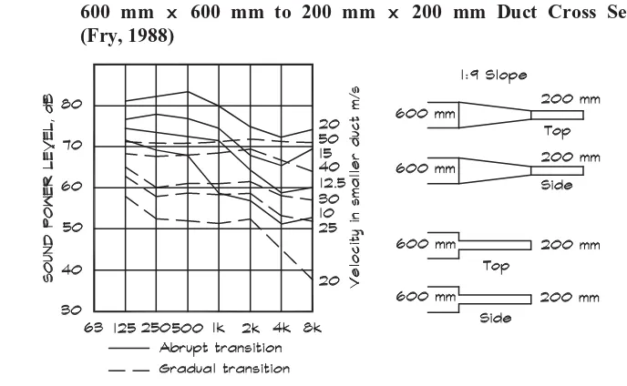
Figure13.19 Sound Power Levels of Abrupt and Gradual Area Transitions from 600 mm × 600 mm to 200 mm × 200 mm Duct Cross Sections (Fry, 1988)
Table 13.9 gives velocity recommendations appropriate for various NC levels in the receiving space. These include consideration of the attenuation of downstream sections of lined duct. For the lined duct velocities, it is assumed that the remaining ductwork is covered on the inside with a 1” (25 mm) thick fiberglass duct liner or is flex duct.
Noise Generated by Transitions
Aerodynamic noise is generated at both gradual and abrupt changes in duct area. Grad-ual transitions and low velocities generate less turbulence than abrupt transitions and high velocities. Beyond these generalizations there are few models to use for sound power level prediction. Fry (1988) has published measured data for several expansion ratios in rectangular ducts, which are reproduced in Figs. 13.19 and 13.20.
Air Generated Noise in Junctions and Turns
Noise generated in transition elements such as turns, elbows, junctions, and takeoffs can run 10 to 20 dB higher than the sound power levels generated in straight duct runs. Ducts having radiused bends, with an aspect ratio of 1:3 generated, no more noise than a straight duct (Fry, 1988). Elbows having a 90◦bend are about 10 dB noisier than straight duct. One or more turning vanes can reduce the noise 8 to 10 dB at high and low frequencies while increasing it 3 to 4 dB in the mid frequencies.
Ver (1984) published an empirical equation for the sound power levels given off by various fittings, which was reproduced in the 1987 ASHRAE guide. For branches, turns (including elbows without turning vanes), and junctions such as those pictured in Fig. 13.21, it is
LW OCT(f0)=KJ+10 log(f0/63)+50 log(UB)+10 log(SB)
Figure13.20 Sound Power Levels of Abrupt and Gradual Area Transitions from 600 mm × 600 mm to 600 mm × 200 mm Duct Cross Sections (Fry, 1988)
Figure13.21 Elbows, Junctions, and Branch Takeoffs
where LW OCT =octave band sound power level (dB re 10−12Watts) f0 =center frequency of the octave band (Hz)
KJ =characteristic spectrum of the junction or turn, based on the Strouhal number
UB =velocity in the branch duct (ft/s)
SB =cross sectional area of the branch duct (ft2)
DB =equivalent diameter of the branch duct or in the case of junctions, DB =
4 SB/π (ft)
CB =a constant which depends on the type of branch or junction The flow velocity in the branch is calculated using
UB =QB/(60 SB) (ft/s) (13.6)
The termr is a correction for the roundness of the bend or elbow associated with the
12 DB for the radius, R (inches), of the inside edge of the bend, and St =f0DB/UB is the Strouhal number.
The termT is a correction for upstream turbulence, which is applied only when there are dampers, elbows, or branch takeoffs upstream, and within five main duct diameters, of the turn or junction under consideration.
T= −1.667+1.8m−0.133m2 (13.8)
m=U
M/UB (13.9)
where UM =velocity in the main duct (ft/min) UB =velocity in the branch duct (ft/min)
The characteristic spectrum KJin Eq. 13.5 may be calculated (Reynolds, 1990) using
KJ = −21.61+12.388m0.673
B depends on the type of junction in Fig. 13.21.
For X - junctions
For 90◦elbows without turning vanes,
C
B =0 (13.13)
For a 90◦branch takeoff,
Air Generated Noise in Dampers
Damper noise follows the same general spectrum equation (Eq. 13.5) as was used for branches and turns, although the terms are defined somewhat differently
LW OCT(f0)=KD +10 log(f0/63)+50 log(UC)
+10 log(S)+10 log(DH)+C D
(13.15)
where LW OCT =octave band sound power level (dB re 10−12Watts) f0 =center frequency of the octave band (Hz)
KD=characteristic spectrum of the damper, based on the pressure loss
factor and the Strouhal number
UC =flow velocity in the constricted part of the duct (ft/s) S=cross sectional area of the branch duct (ft2)
DH =duct height normal to the damper axis (ft)
Before solving Eq. 13.15, several preliminary calculations must be undertaken. The charac-teristic spectrum is determined from the Strouhal number, which depends on the velocity, the blockage factor, and the pressure loss coefficient, C.
The pressure loss coefficient in FP units is
C=15.9·106 P
(Q/S)2 (13.16)
where P=pressure drop across the fitting (in. w.g.) Q=flow volume, (cfm)
The blockage factor, B, for multiblade dampers and elbows with turning vanes is
B=
For single blade dampers, it is
B=
Next the constricted velocity is calculated using
which gives the Strouhal number
St =f0 D/Uc (13.22)
Having calculated these numbers for the particular fitting we can find the characteristic spectrum for dampers (Reynolds, 1990)
KD = −36.6−10.7 log(St) for St ≤25
KD = −1.1−35.9 log(St) for St >25 (13.23)
Air Noise Generated by Elbows with Turning Vanes
For elbows with turning vanes we use Ver’s equation with a slightly different definition of the terms
LW OCT(f0)=KT+10 log(f0/63)+50 log(UC)
+10 log(S)+10 log(DC)+10 log n (13.24)
where LW OCT =octave band sound power level (dB re 10−12Watts) f0 =center frequency of the octave band (Hz)
KT =characteristic spectrum of an elbow with turning vanes UC =flow velocity in the constricted part of the flow field (ft/s)
S=cross sectional area of the elbow (ft2) DC =chord length of a typical vane (in)
n=number of turning vanes
Figure 13.22 shows the definition of the chord length. The characteristic spectrum (Reynolds, 1990) is
KT = −47.5−7.69 [log(St)]2.5 (13.25)
where the Strouhal number in Eq. 13.22 is calculated from the pressure loss coefficient in Eq. 13.16, the blockage factor,
B= √
C−1
C−1 (13.26)
and the constricted velocity in Eq. 13.21.
Grilles, Diffusers, and Integral Dampers
Diffuser generated noise is of paramount importance in HVAC noise control since it cannot be attenuated by the addition of downstream devices. Since diffuser noise is primarily dependent on the air velocity through the device, the only method for attenuating it is to reduce it, either by adding additional diffusers, or by increasing the size of the existing diffusers. Often diffuser noise is influenced by the upstream flow conditions that can be modified. Pressure equalizing grilles at the entry to the diffuser can help reduce the contribution due to turbulence.
Sound data on diffuser noise is published by manufacturers in terms of NC levels; however, these are only valid for ideal flow conditions. To achieve ideal conditions, flexible ducts must be straight for at least one duct diameter before the connection to the diffuser and must not be pinched or constricted. Figure 13.23 shows examples of correct and incorrect flexible duct connections.
It should be noted that manufacturer published data are given for one diffuser or, in the case of linear diffusers, for one four-foot long segment, with a power-to-pressure conversion of 10 dB, which corresponds to a room absorption of about 400 sabins and a distance of about 12 ft. The actual power-to-pressure conversion factor should be calculated for the specific room in question. Where there are multiple diffusers in a space, a factor of 10 log n, where n is the number of diffusers or the total number of four-foot segments of linear diffuser, must be added to the published noise levels.
When sound levels from diffusers are not available, they can be approximated using a general equation (Reynolds, 1990). It relates the diffuser noise to the sixth power of the flow
velocity and the third power of the pressure drop.
Lw =10 log SG +30 logξ +60 log UG−31.3 (13.27)
where LW =overall sound power level (dB re 10−12 Watts) SG =cross sectional face area of the grille or diffuser (ft2) UG =flow velocity prior to the diffuser (ft/s)
ξ =normalized pressure drop coefficient
It is clear that the noise emitted by diffusers is very dependent on the flow velocity and the formula yields an 18 dB per doubling of velocity relationship. For a given flow volume a doubling of grill area will reduce noise by 15 dB.
The normalized pressure drop is
ξ =334.9 P
ρ0 U2
G
(13.28)
where P=pressure drop across the diffuser (in w.g.) ρ0 =density of air (0.075 lb/ft3)
UG =flow velocity prior to the diffuser (ft/min)
= 60 SQ
G
(for Q in cfm)
The octave band sound power levels can be calculated from the overall level by adding a correction factor to Eq. 13.27
LW OCT =LW+CD (13.29)
The correction term for round diffusers is
CD = −5.82−0.15A−1.13 A2 (13.30)
and for rectangular (including slot) diffusers,
CD = −11.82−0.15A−1.13 A2 (13.31)
and is normalized to a peak frequency
fP =48.8 UG (13.32)
The term A is
A=NB (fP)−NB (f) (13.33)
Figure13.24 Generalized Shape of the Diffuser Spectrum (ASHRAE, 1995)
Dampers located close to an outlet diffuser can add appreciably to the noise generated by the termination. First the damper generates vortex shedding in its wake, which is a source of noise. Second, downstream turbulence increases the noise generated by the grille. Manufacturers of these devices can provide sound power levels for a given flow volume. If these are not available it can be assumed that levels will increase 5 dB in all bands with the dampers in the fully open position. As the dampers are closed, there is an increase in the pressure drop across the damper, which restricts the flow. The overall sound power level increases approximately as (Fry, 1988)
Lw =33 log(P/P0) (13.34)
where LW =increase in sound power level radiated by the diffuser (dB) P=new static pressure drop across the unit (in. w.g.)
P0 =initial static pressure drop with the damper in place but with the vanes fully open with the same flow volume (in. w.g.)
Figure 13.25 shows the effect of integral dampers on noise radiated by ceiling diffusers for various settings. For dampers and grills to act as separate sources they should be located at least 4 duct diameters apart.
13.5 NOISE FROM OTHER MECHANICAL EQUIPMENT Air Compressors
Figure13.25 Ceiling Diffuser Damper—Sound Power Spectra (Fry, 1988)
Figure13.26 Sound Pressure Levels of Air Compressors at a Distance of 3 Feet (Miller, 1980)
Transformers
Table13.10 Level Adjustments for the NEMA Rating of a Transformer, dB (Miller, 1980)
Octave Band Center Frequency, Hz
31 63 125 250 500 1k 2k 4k 8k
CT -1 5 7 2 2 -4 -9 -14 -21
through a string tied around the unit), and the correction term, which includes the 10.5 dB adjustment for the power to pressure conversion. Table 13.10 gives the correction term for an unenclosed transformer.
Lw =NEMA rating+10 log ST+CT (13.35)
where Lw OCT =octave band sound pressure level (dB) ST=surface area of the transformer (ft2) CT=octave band correction (dB)
Over time, transformers can grow noisier as their laminations and tie bolts become loose. Miller cites increases as large as 5 dB at the fundamental and 10 dB in the second and third harmonic frequencies. When transformers are enclosed in small vaults they can induce standing wave patterns in the room, which have the effect of increasing the transmitted power by 6 dB in the same bands.
Transformers that are directly tied to a wall can induce structure-borne noise. Jones (1984) recommends isolation techniques shown in Fig. 13.27 to prevent this. In areas of seismic activity, one or more sway braces may be necessary to provide stability at the top of the unit.
Reciprocating Engines and Emergency Generators
Most large buildings have emergency generators to provide power when the normal sources fail. It is often argued that noise control of emergency generators is unnecessary since they would be used only in an emergency, when noise is a secondary concern. Although this is probably true, generators must be tested periodically, an hour a month, and during these test periods the building functions normally and noise is still a concern. During power outages generators can be needed over longer periods of time.
Generator sets are powered by a diesel, methane, or propane fuel reciprocating engine and radiate sound from their casing, intake, and exhaust. Miller (1980) measured the casing radiated power levels, which followed the relationship
Lw =93+10 log(rated hp)+A+B+C+D (13.36)
where Lw =overall sound power level (dB)
rated hp=engine manufacturer’s continuous full load rating for the engine, (horse power)
A, B, C, D=correction terms given in Table 13.11 (dB)
Figure13.27 Vibration Isolation of Floor-Mounted Transformers (Jones, 1984)
Table13.11 Level Adjustments for Engine Casing Radiated Noise, dB (Miller, 1980)
Speed Correction Term, A
Under 600 rpm −5
600 - 1500 rpm −2
Above 1500 rpm 0
Fuel Correction Term, B
Diesel fuel only 0
Diesel and/or natural gas 0
Natural gas only (may have small amounts of “pilot oil”) −3 Cylinder Arrangement Term, C
In-line 0
V-type −1
Radial −1
Air Intake Correction Term, D
Unducted air inlet to unmuffled Roots Blower +3 Ducted air from outside the room or into muffled Roots Blower 0 All other inlets to engine (with or without turbochargers) 0
Noise radiated from the inlet is usually the same as the casing radiation unless there is a separate ducted inlet to a turbocharger. In these cases the inlet noise is given by
Table13.12 Frequency Adjustments for Casing Radiated Noise of Reciprocating Engines (Miller, 1980)
Value to be Subtracted from Sound Power Level, dB Engine Speed 600-1500 rpm
Octave
Frequency Engine Engine
Band Speed Without With Speed
(Hz) Under Roots Roots Over
600 rpm Blower Blower 1500 rpm
31 12 14 22 22
Table13.13 Level Adjustments for Turbocharger Air Inlet, dB (Miller, 1980)
Octave Band Center Frequency (Hz)
31 63 125 250 500 1k 2k 4k 8k A
Correction 4 11 13 13 12 9 8 9 17 3
Any losses due to inlet ductwork or silencers must be subtracted from the octave band sound power levels. The corrections for each octave band are given in Table 13.13 and are subtracted from the overall sound power level.
The exhaust is the loudest source. The overall sound power level for noise radiated from an unmuffled engine exhaust is
Lw =119+10 log(rated hp)−T (13.38)
where the factor T is the turbocharger correction term (T=0 dB for no turbocharger and T=6 dB for an engine with a turbocharger). The effects of any downstream exhaust pip-ing or mufflers must be subtracted from the sound power level in each band. Octave-band adjustments to be subtracted form the overall sound power level are shown in Table 13.14.
Table13.14 Level Adjustments for Engine Exhaust, dB (Miller, 1980)
Octave Band Center Frequency (Hz)
31 63 125 250 500 1k 2k 4k 8k A