OVERVIEW The concept of a limit is a central idea that distinguishes calculus from alge-bra and trigonometry. It is fundamental to finding the tangent to a curve or the velocity of an object.
In this chapter we develop the limit, first intuitively and then formally. We use limits to describe the way a function ƒ varies. Some functions vary continuously; small changes in xproduce only small changes in ƒ(x). Other functions can have values that jump or vary erratically. The notion of limit gives a precise way to distinguish between these behaviors. The geometric application of using limits to define the tangent to a curve leads at once to the important concept of the derivative of a function. The derivative, which we investigate thoroughly in Chapter 3, quantifies the way a function’s values change.
L
IMITS AND
C
ONTINUITY
C h a p t e r
2
Rates of Change and Limits
In this section, we introduce average and instantaneous rates of change. These lead to the main idea of the section, the idea of limit.
Average and Instantaneous Speed
A moving body’s average speedduring an interval of time is found by dividing the dis-tance covered by the time elapsed. The unit of measure is length per unit time: kilometers per hour, feet per second, or whatever is appropriate to the problem at hand.
EXAMPLE 1 Finding an Average Speed
A rock breaks loose from the top of a tall cliff. What is its average speed
(a) during the first 2 sec of fall?
(b) during the 1-sec interval between second 1 and second 2?
the only force acting on the falling body. We call this type of motion free fall.) If ydenotes the distance fallen in feet after tseconds, then Galileo’s law is
where 16 is the constant of proportionality.
The average speed of the rock during a given time interval is the change in distance, divided by the length of the time interval,
(a) For the first 2 sec:
(b) From sec 1 to sec 2:
The next example examines what happens when we look at the average speed of a falling object over shorter and shorter time intervals.
EXAMPLE 2 Finding an Instantaneous Speed
Find the speed of the falling rock at and
Solution We can calculate the average speed of the rock over a time interval having length as
(1)
We cannot use this formula to calculate the “instantaneous” speed at by substituting because we cannot divide by zero. But we canuse it to calculate average speeds over increasingly short time intervals starting at and When we do so, we see a pattern (Table 2.1).
t0 = 2 .
t0 = 1
h = 0 ,
t0 ¢y
¢t =
16st0 + hd2 - 16t02
h .
¢t = h,
[t0, t0 + h] ,
t = 2sec . t = 1
¢y ¢t =
16s2d2 - 16s1d2
2 - 1 = 48
ft sec ¢y
¢t =
16s2d2 - 16s0d2
2 - 0 = 32
ft sec ¢t.
¢y,
y = 16t2,
74
Chapter 2: Limits and ContinuityHISTORICALBIOGRAPHY* Galileo Galilei
(1564–1642)
TABLE 2.1 Average speeds over short time intervals
Length of Average speed over Average speed over time interval interval of length h interval of length h
h starting at starting at
1 48 80
0.1 33.6 65.6
0.01 32.16 64.16
0.001 32.016 64.016
0.0001 32.0016 64.0016
t0ⴝ 2 t0ⴝ 1
Average speed: ¢¢y t =
16st0 + hd2 - 16t 02
h
The average speed on intervals starting at seems to approach a limiting value of 32 as the length of the interval decreases. This suggests that the rock is falling at a speed of 32 ft sec at > t0 = 1sec .Let’s confirm this algebraically.
t0 = 1
If we set and then expand the numerator in Equation (1) and simplify, we find that
For values of hdifferent from 0, the expressions on the right and left are equivalent and the average speed is We can now see why the average speed has the limiting
value as happroaches 0.
Similarly, setting in Equation (1), the procedure yields
for values of hdifferent from 0. As hgets closer and closer to 0, the average speed at has the limiting value 64 ft sec.
Average Rates of Change and Secant Lines
Given an arbitrary function we calculate the average rate of change of ywith respect to x over the interval by dividing the change in the value of y,
by the length of the interval over which the
change occurs.
¢x = x2 - x1 = h ¢y = ƒsx2d - ƒsx1d,
[x1, x2]
y = ƒsxd, > t0 = 2sec
¢y
¢t = 64 + 16h t0 = 2
32 + 16s0d = 32 ft>sec 32 + 16h ft>sec .
= 32h + 16h2
h = 32 + 16h. ¢y
¢t =
16s1 + hd2 - 16s1d2
h =
16s1 + 2h + h2d - 16 h
t0 = 1
2.1 Rates of Change and Limits
75
DEFINITION Average Rate of Change over an Interval
Theaverage rate of changeof with respect toxover the interval is ¢y
¢x =
ƒsx2d - ƒsx1d
x2 - x1 =
ƒsx1 + hd - ƒsx1d
h , h Z 0 .
[x1, x2]
y = ƒsxd
Geometrically, the rate of change of ƒ over is the slope of the line through the points and (Figure 2.1). In geometry, a line joining two points of a curve is a secantto the curve. Thus, the average rate of change of ƒ from to is iden-tical with the slope of secant PQ.
Experimental biologists often want to know the rates at which populations grow under controlled laboratory conditions.
EXAMPLE 3 The Average Growth Rate of a Laboratory Population
Figure 2.2 shows how a population of fruit flies (Drosophila) grew in a 50-day experi-ment. The number of flies was counted at regular intervals, the counted values plotted with respect to time, and the points joined by a smooth curve (colored blue in Figure 2.2). Find the average growth rate from day 23 to day 45.
Solution There were 150 flies on day 23 and 340 flies on day 45. Thus the number of
flies increased by in days. The average rate of change
of the population from day 23 to day 45 was Average rate of change: ¢¢p
t =
340 - 150 45 - 23 =
190
22 L 8.6 flies>day . 45 - 23 = 22
340 - 150 = 190
x2
x1
Qsx2, ƒsx2dd
Psx1, ƒsx1dd
[x1, x2]
y
x
0
Secant
P(x1, f(x1))
Q(x2, f(x2))
⌬x ⫽ h
⌬y
x2
x1
y⫽f(x)
FIGURE 2.1 A secant to the graph
Its slope is the
average rate of change of ƒ over the interval [x1, x2] .
This average is the slope of the secant through the points Pand Qon the graph in Figure 2.2.
The average rate of change from day 23 to day 45 calculated in Example 3 does not tell us how fast the population was changing on day 23 itself. For that we need to examine time intervals closer to the day in question.
EXAMPLE 4 The Growth Rate on Day 23
How fast was the number of flies in the population of Example 3 growing on day 23?
Solution To answer this question, we examine the average rates of change over increas-ingly short time intervals starting at day 23. In geometric terms, we find these rates by cal-culating the slopes of secants from Pto Q, for a sequence of points Qapproaching Palong the curve (Figure 2.3).
76
Chapter 2: Limits and Continuityt p
10
0 20 30 40 50
50 100 150 200 250 300 350
P(23, 150)
Q(45, 340)
⌬t ⫽22
⌬p ⫽190
⌬t
⌬p
⬇ 8.6 flies/day
Time (days)
Number of flies
FIGURE 2.2 Growth of a fruit fly population in a controlled
experiment. The average rate of change over 22 days is the slope of the secant line.
¢p>¢t
t
Number
of
flies
p
350
300
250
200
150
100
50
0 10 20 30 40 50
Time (days)
Number of flies
A(14, 0)
P(23, 150)
B(35, 350)
Q(45, 340)
FIGURE 2.3 The positions and slopes of four secants through the point Pon the fruit fly graph (Example 4).
Slope of
Q (flies day)
(45, 340)
(40, 330)
(35, 310)
(30, 265) 265 - 150 30 - 23 L 16.4 310 - 150
35 - 23 L 13.3 330 - 150
40 - 23 L 10.6 340 - 150
45 - 23 L 8.6 /
The values in the table show that the secant slopes rise from 8.6 to 16.4 as the t-coor-dinate of Qdecreases from 45 to 30, and we would expect the slopes to rise slightly higher as tcontinued on toward 23. Geometrically, the secants rotate about P and seem to ap-proach the red line in the figure, a line that goes through Pin the same direction that the curve goes through P. We will see that this line is called the tangentto the curve at P. Since the line appears to pass through the points (14, 0) and (35, 350), it has slope
(approximately).
On day 23 the population was increasing at a rate of about 16.7 flies day. The rates at which the rock in Example 2 was falling at the instants and and the rate at which the population in Example 4 was changing on day are called instantaneous rates of change. As the examples suggest, we find instantaneous rates as limiting values of average rates. In Example 4, we also pictured the tangent line to the pop-ulation curve on day 23 as a limiting position of secant lines. Instantaneous rates and tan-gent lines, intimately connected, appear in many other contexts. To talk about the two con-structively, and to understand the connection further, we need to investigate the process by which we determine limiting values, or limits, as we will soon call them.
Limits of Function Values
Our examples have suggested the limit idea. Let’s begin with an informal definition of limit, postponing the precise definition until we’ve gained more insight.
Let ƒ(x) be defined on an open interval about except possibly at itself. If ƒ(x) gets arbitrarily close to L(as close to Las we like) for all xsufficiently close to we say that ƒ approaches the limitLas xapproaches and we write
which is read “the limit of ƒ(x) as xapproaches is L”. Essentially, the definition says that the values of ƒ(x) are close to the number Lwhenever xis close to (on either side of ). This definition is “informal” because phrases likearbitrarily closeand sufficiently closeare imprecise; their meaning depends on the context. To a machinist manufacturing a piston, closemay mean within a few thousandths of an inch. To an astronomer studying distant galaxies,closemay meanwithin a few thousand light-years. The definition is clear enough, however, to enable us to recognize and evaluate limits of specific functions. We will need the precise definition of Section 2.3, however, when we set out to prove theorems about limits.
EXAMPLE 5 Behavior of a Function Near a Point
How does the function
behave near
Solution The given formula defines ƒ for all real numbers xexcept (we cannot di-vide by zero). For any we can simplify the formula by factoring the numerator and canceling common factors:
ƒsxd = sx - 1dsx + 1d
x - 1 = x + 1 for x Z 1 . x Z 1 ,
x = 1 x = 1 ?
ƒsxd = x2 - 1 x - 1
x0
x0
x0
lim x:x0 ƒsxd
= L, x0,
x0,
x0
x0,
t = 23
t = 2 t = 1
> 350 - 0
35 - 14 = 16.7 flies>day
The graph of ƒ is thus the line with the point (1, 2) removed. This removed point is shown as a “hole” in Figure 2.4. Even though ƒ(1) is not defined, it is clear that we can make the value of ƒ(x) as close as we wantto 2 by choosing x close enoughto 1 (Table 2.2).
y = x + 1
78
Chapter 2: Limits and Continuityx y
0 1
2
1
x y
0 1
2
1 y⫽f(x) ⫽
x2⫺ 1
x⫺ 1
y⫽x⫹ 1 –1
–1
FIGURE 2.4 The graph of ƒ is
identical with the line
except at where ƒ is not
defined (Example 5). x = 1 ,
y = x + 1
x2⫺ 1
x⫺ 1
x y
0 1
2
1
x y
0 1
2
1
x y
0 1
–1 –1
–1
2
1
1,
, (a) f(x) ⫽x2⫺ 1 (b) g(x) ⫽
x⫺ 1
x⫽ 1
x⫽ 1
(c) h(x) ⫽x⫹ 1
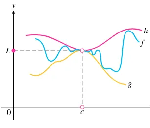
FIGURE 2.5 The limits of ƒ (x), g(x), and h(x) all equal 2 as xapproaches 1. However,
only h(x) has the same function value as its limit at x = 1(Example 6).
TABLE 2.2 The closer xgets to 1, the closer ƒ(x)⫽(x2⫺1)/(x⫺1)
seems to get to 2
Values of xbelow and above 1 ƒ(x) ⴝ
0.9 1.9
1.1 2.1
0.99 1.99
1.01 2.01
0.999 1.999
1.001 2.001
0.999999 1.999999
1.000001 2.000001
x2ⴚ 1
xⴚ 1 ⴝxⴙ 1, xⴝ 1
We say that ƒ(x) approaches the limit2 as xapproaches 1, and write
EXAMPLE 6 The Limit Value Does Not Depend on How the Function Is
Defined at
The function ƒ in Figure 2.5 has limit 2 as even though ƒ is not defined at The function ghas limit 2 as x:1even though 2 Z gs1d.The function his the only one
x = 1 . x:1
x0 lim
x:1 ƒsxd = 2, or xlim:1 x2 - 1
whose limit as equals its value at For h, we have This equality of limit and function value is special, and we return to it in Section 2.6.
Sometimes can be evaluated by calculating This holds, for exam-ple, whenever ƒ(x) is an algebraic combination of polynomials and trigonometric func-tions for which is defined. (We will say more about this in Sections 2.2 and 2.6.)
EXAMPLE 7 Finding Limits by Calculating ƒ(x0)
(a)
(b)
(c)
(d)
(e)
EXAMPLE 8 The Identity and Constant Functions Have Limits at Every Point
(a) If ƒ is the identity function then for any value of (Figure 2.6a),
(b) If ƒ is the constant function (function with the constant value k), then for any value of (Figure 2.6b),
For instance,
We prove these results in Example 3 in Section 2.3.
Some ways that limits can fail to exist are illustrated in Figure 2.7 and described in the next example.
2.1 Rates of Change and Limits
79
(a) Identity function
(b) Constant function 0
FIGURE 2.6 The functions in Example 8.
x
EXAMPLE 9 A Function May Fail to Have a Limit at a Point in Its Domain Discuss the behavior of the following functions as
(a)
(b)
(c)
Solution
(a) It jumps:The unit step functionU(x) has no limit as because its values jump at For negative values of xarbitrarily close to zero, For positive values of xarbitrarily close to zero, There is no singlevalue Lapproached by U(x) as (Figure 2.7a).
(b) It grows too large to have a limit: g(x) has no limit as because the values of g grow arbitrarily large in absolute value as and do not stay close to anyreal number (Figure 2.7b).
(c) It oscillates too much to have a limit: ƒ(x) has no limit as because the function’s values oscillate between and in every open interval containing 0. The values do not stay close to any one number as (Figure 2.7c).
Using Calculators and Computers to Estimate Limits
Tables 2.1 and 2.2 illustrate using a calculator or computer to guess a limit numerically as xgets closer and closer to That procedure would also be successful for the limits of functions like those in Example 7 (these are continuousfunctions and we study them in Section 2.6). However, calculators and computers can give false values and misleading im-pressionsfor functions that are undefined at a point or fail to have a limit there. The differ-ential calculus will help us know when a calculator or computer is providing strange or ambiguous information about a function’s behavior near some point (see Sections 4.4 and 4.6). For now, we simply need to be attentive to the fact that pitfalls may occur when using computing devices to guess the value of a limit. Here’s one example.
EXAMPLE 10 Guessing a Limit
Guess the value of
Solution Table 2.3 lists values of the function for several values near As x
ap-proaches 0 through the values and the function seems to
ap-proach the number 0.05.
As we take even smaller values of x, and the function appears to approach the value 0.
So what is the answer? Is it 0.05 or 0, or some other value? The calculator/computer values are ambiguous, but the theorems on limits presented in the next section will con-firm the correct limit value to be 0.05
A
= 1冫20B
.Problems such as these demonstrate the ;0.000001 , ;0.0005, ;0.0001, ;0.00001 ,;0.01 , ;1, ;0.5, ;0.10 ,
x = 0 . lim
x:0
2x2 + 100 - 10
x2 .
x0.
x:0 -1
+1
x:0 x:0
x:0 x:0
Usxd = 1 .
Usxd = 0 . x = 0 .
x:0 ƒsxd = •0, x … 0
sin1x, x 7 0 gsxd = L
1
x, x Z 0 0, x = 0 Usxd = e0, x 6 0 1, x Ú 0
power of mathematical reasoning, once it is developed, over the conclusions we might draw from making a few observations. Both approaches have advantages and disadvan-tages in revealing nature’s realities.
2.1 Rates of Change and Limits
81
TABLE 2.3 Computer values of ƒ(x) ⫽ Near x⫽0
x ƒ(x)
;0.0005 0.080000
;0.0001 0.000000
;0.00001 0.000000 ;0.000001 0.000000
t approaches 0 ?
;1 0.049876
;0.5 0.049969
;0.1 0.049999
;0.01 0.050000
t approaches 0.05 ?
2x2+ 100 - 10
2.1 Rates of Change and Limits
81
EXERCISES 2.1
Limits from Graphs
1. For the function g(x) graphed here, find the following limits or explain why they do not exist.
a. b. c.
2. For the function ƒ(t) graphed here, find the following limits or ex-plain why they do not exist.
a. b. c.
t s
1
1 0
s⫽f(t)
–1 –1
–2
lim
t:0 ƒstd
lim
t:-1 ƒstd
lim
t:-2 ƒstd
3 x
y
2 1
1
y⫽g(x)
lim
x:3gsxd
lim
x:2gsxd
lim
x:1gsxd
3. Which of the following statements about the function graphed here are true, and which are false?
a. exists.
b.
c.
d.
e.
f. exists at every point in
4. Which of the following statements about the function graphed here are true, and which are false?
a. does not exist.
b. lim
x:2 ƒsxd = 2 .
lim
x:2 ƒsxd
y = ƒsxd
x y
2 1 –1
1
–1
y⫽f(x) s-1, 1d. x0
lim
x:x0 ƒsxd lim
x:1 ƒsxd = 0 .
lim
x:1 ƒsxd = 1 .
lim
x:0 ƒsxd = 1 .
lim
x:0 ƒsxd = 0 .
lim
x:0 ƒsxd
c. does not exist.
d. exists at every point in
e. exists at every point in (1, 3).
Existence of Limits
In Exercises 5 and 6, explain why the limits do not exist.
5. 6.
7. Suppose that a function ƒ(x) is defined for all real values of x
ex-cept Can anything be said about the existence of
Give reasons for your answer.
8. Suppose that a function ƒ(x) is defined for all xin Can
anything be said about the existence of Give
rea-sons for your answer.
9. If must ƒ be defined at If it is, must
Can we conclude anything about the values of ƒ at Explain.
10. If must exist? If it does, then must
Can we conclude anythingabout Explain.
Estimating Limits
You will find a graphing calculator useful for Exercises 11–20. 11. Let
a. Make a table of the values of ƒ at the points
and so on as far as your calculator can go.
Then estimate What estimate do you arrive at if
you evaluate ƒ at instead?
b. Support your conclusions in part (a) by graphing ƒ near and using Zoom and Trace to estimate y-values on the graph as
c. Find algebraically, as in Example 5.
12. Let
a. Make a table of the values of gat the points
and so on through successive decimal approximations of Estimate
b. Support your conclusion in part (a) by graphing gnear and using Zoom and Trace to estimate y-values on the graph as
and so on. Then estimate What estimate do you
arrive at if you evaluate Gat instead?
b. Support your conclusions in part (a) by graphing Gand using Zoom and Trace to estimate y-values on the graph as
c. Find algebraically.
14. Let
a. Make a table of the values of hat and so
on. Then estimate What estimate do you arrive
at if you evaluate hat instead?
b. Support your conclusions in part (a) by graphing hnear and using Zoom and Trace to estimate y-values on the graph as
c. Find algebraically.
15. Let
a. Make tables of the values of ƒ at values of xthat approach from above and below. Then estimate
b. Support your conclusion in part (a) by graphing ƒ near and using Zoom and Trace to estimate y-values on the graph as
c. Find algebraically.
16. Let
a. Make tables of values of Fat values of xthat approach from above and below. Then estimate b. Support your conclusion in part (a) by graphing Fnear
and using Zoom and Trace to estimate y-values on the graph as
c. Find algebraically.
17. Let
a. Make a table of the values of gat values of that approach from above and below. Then estimate
b. Support your conclusion in part (a) by graphing gnear
18. Let
a. Make tables of values of Gat values of tthat approach from above and below. Then estimate
b. Support your conclusion in part (a) by graphing Gnear
19. Let
a. Make tables of values of ƒ at values of xthat approach from above and below. Does ƒ appear to have a limit as
If so, what is it? If not, why not?
b. Support your conclusions in part (a) by graphing ƒ near x0= 1 .
82
Chapter 2: Limits and Continuity20. Let
a. Make tables of values of ƒ at values of xthat approach from above and below. Does ƒ appear to have a limit as
If so, what is it? If not, why not?
b. Support your conclusions in part (a) by graphing ƒ near
Limits by Substitution
In Exercises 21–28, find the limits by substitution. Support your an-swers with a computer or calculator if available.
21. 22.
23. 24.
25. 26.
27. 28.
Average Rates of Change
In Exercises 29–34, find the average rate of change of the function over the given interval or intervals.
29.
35. A Ford Mustang Cobra’s speed The accompanying figure
shows the time-to-distance graph for a 1994 Ford Mustang Cobra accelerating from a standstill.
0 5
200
100
Elapsed time (sec)
Distance (m)
arranging them in order in a table like the one in Figure 2.3. What are the appropriate units for these slopes?
b. Then estimate the Cobra’s speed at time
36. The accompanying figure shows the plot of distance fallen versus time for an object that fell from the lunar landing module a dis-tance 80 m to the surface of the moon.
a. Estimate the slopes of the secants and
arranging them in a table like the one in Figure 2.3. b. About how fast was the object going when it hit the surface?
37. The profits of a small company for each of the first five years of its operation are given in the following table:
a. Plot points representing the profit as a function of year, and join them by as smooth a curve as you can.
b. What is the average rate of increase of the profits between 1992 and 1994?
c. Use your graph to estimate the rate at which the profits were changing in 1992.
38. Make a table of values for the function at the points
and
a. Find the average rate of change of F(x) over the intervals [1, x] for each in your table.
b. Extending the table if necessary, try to determine the rate of change of F(x) at
39. Let for
a. Find the average rate of change of g(x) with respect to xover the intervals [1, 2], [1, 1.5] and
b. Make a table of values of the average rate of change of gwith respect to xover the interval [1, 1+ h]for some values of h
Year Profit in $1000s
1990 6
Elapsed time (sec)
Distance fallen (m)
5 10
2.1 Rates of Change and Limits
83
T
T
84
Chapter 2: Limits and Continuityapproaching zero, say and 0.000001.
c. What does your table indicate is the rate of change of g(x) with respect to xat
d. Calculate the limit as happroaches zero of the average rate of change of g(x) with respect to xover the interval
40. Let for
a. Find the average rate of change of ƒ with respect to tover the
intervals (i) from to and (ii) from to
b. Make a table of values of the average rate of change of ƒ with respect to tover the interval [2, T], for some values of T approaching 2, say
and 2.000001.
c. What does your table indicate is the rate of change of ƒ with respect to tat t = 2 ?
T= 2.1, 2.01, 2.001, 2.0001, 2.00001 , t = T.
t = 2 t= 3 ,
t = 2 t Z 0 . ƒstd = 1>t
[1, 1 + h] . x = 1 ?
h = 0.1, 0.01, 0.001, 0.0001, 0.00001 , d. Calculate the limit as Tapproaches 2 of the average rate of change of ƒ with respect to tover the interval from 2 to T. You will have to do some algebra before you can substitute
COMPUTER EXPLORATIONS
Graphical Estimates of Limits
In Exercises 41–46, use a CAS to perform the following steps: a. Plot the function near the point being approached. b. From your plot guess the value of the limit.
41. 42.
43. 44.
45. 46. lim
x:0
2x2 3 - 3cosx lim
x:0
1 - cosx
xsinx
lim
x:3
x2 - 9 2x2 + 7 - 4 lim
x:0
231 +
x - 1
x
lim
x:-1
x3- x2- 5x - 3 sx + 1d2 lim
x:2
x4 - 16
x - 2
x0
T= 2 .
84
Chapter 2: Limits and ContinuityCalculating Limits Using the Limit Laws
In Section 2.1 we used graphs and calculators to guess the values of limits. This section presents theorems for calculating limits. The first three let us build on the results of Exam-ple 8 in the preceding section to find limits of polynomials, rational functions, and powers. The fourth and fifth prepare for calculations later in the text.
The Limit Laws
The next theorem tells how to calculate limits of functions that are arithmetic combina-tions of funccombina-tions whose limits we already know.
2.2
HISTORICALESSAY*
Limits
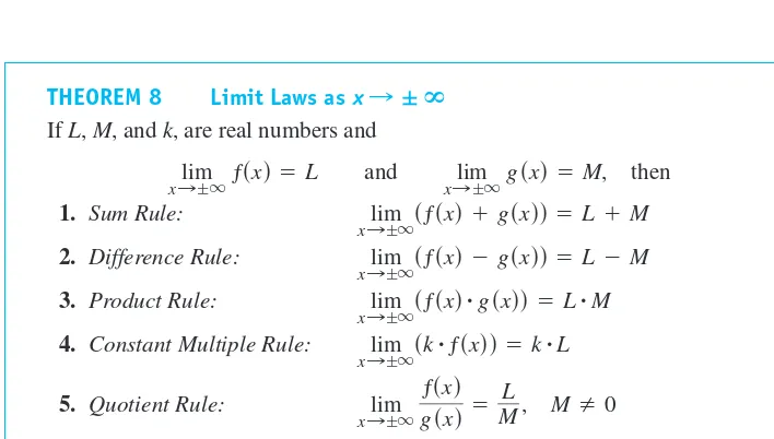
THEOREM 1 Limit Laws
If L,M,cand kare real numbers and
1. Sum Rule:
The limit of the sum of two functions is the sum of their limits.
2. Difference Rule:
The limit of the difference of two functions is the difference of their limits.
3. Product Rule:
The limit of a product of two functions is the product of their limits. lim
x:csƒsxd
#
gsxdd = L#
M limx:csƒsxd - gsxdd = L - M lim
x:csƒsxd + gsxdd = L + M lim
x:c ƒsxd = L and xlim:c gsxd = M, then
It is easy to convince ourselves that the properties in Theorem 1 are true (although these intuitive arguments do not constitute proofs). If xis sufficiently close to c, then ƒ(x) is close to Land g(x) is close to M, from our informal definition of a limit. It is then
rea-sonable that is close to is close to ƒ(x)g(x) is
close to LM; kƒ(x) is close to kL; and that is close to if Mis not zero. We prove the Sum Rule in Section 2.3, based on a precise definition of limit. Rules 2–5 are proved in Appendix 2. Rule 6 is proved in more advanced texts.
Here are some examples of how Theorem 1 can be used to find limits of polynomial and rational functions.
EXAMPLE 1 Using the Limit Laws
Use the observations and (Example 8 in Section 2.1) and the
properties of limits to find the following limits.
(a) (b) (c)
Solution
(a) Sum and Difference Rules
Product and Multiple Rules
(b) Quotient Rule
Sum and Difference Rules
Power or Product Rule = c4 + c2 - 1
c2 + 5 =
lim x:c x
4 + lim
x:c x
2 - lim
x:c 1 lim
x:c x
2 + lim
x:c 5 lim
x:c
x4 + x2 - 1 x2 + 5 =
lim x:csx
4 + x2 - 1d
lim x:csx
2 + 5d = c3 + 4c2 - 3 lim
x:csx
3 + 4x2 - 3d = lim
x:c x
3 + lim
x:c 4x
2 - lim
x:c 3
lim x:-2
24x2 - 3 lim
x:c
x4 + x2 - 1 x2 + 5 lim
x:csx
3 + 4x2 - 3d
limx:c x = c
limx:c k = k
L>M ƒ(x)>g(x)
L - M; L + M; ƒsxd - gsxd
ƒsxd + gsxd
2.2 Calculating Limits Using the Limit Laws
85
4. Constant Multiple Rule:
The limit of a constant times a function is the constant times the limit of the function.
5. Quotient Rule:
The limit of a quotient of two functions is the quotient of their limits, provided the limit of the denominator is not zero.
6. Power Rule: If rand sare integers with no common factor and then
provided that is a real number. (If sis even, we assume that )
The limit of a rational power of a function is that power of the limit of the func-tion, provided the latter is a real number.
L 7 0 . Lr>s
lim x:csƒsxdd
r>s = Lr>s
s Z 0 , lim
x:c ƒsxd gsxd =
L
M, M Z 0 lim
x:csk
(c)
Difference Rule
Product and Multiple Rules
Two consequences of Theorem 1 further simplify the task of calculating limits of polyno-mials and rational functions. To evaluate the limit of a polynomial function as x ap-proaches c, merely substitute cfor xin the formula for the function. To evaluate the limit of a rational function as xapproaches a point c at which the denominator is not zero, sub-stitute cfor xin the formula for the function. (See Examples 1a and 1b.)
= 213 = 216 - 3 = 24s-2d2 - 3 = 2 lim
x:-2 4x
2 - lim
x:-2 3
Power Rule with r>s= 1冫 2 lim
x:-2
24x2 - 3 = 2 lim
x:-2
s4x2 - 3d
86
Chapter 2: Limits and ContinuityTHEOREM 2 Limits of Polynomials Can Be Found by Substitution If then
lim
x:c Psxd = Pscd = anc
n + a
n-1cn-1 + Á + a0.
Psxd = anxn + an-1xn-1 + Á + a0,
THEOREM 3 Limits of Rational Functions Can Be Found by Substitution If the Limit of the Denominator Is Not Zero
If P(x) and Q(x) are polynomials and then
lim x:c
Psxd Qsxd =
Pscd Qscd. Qscd Z 0 ,
EXAMPLE 2 Limit of a Rational Function
This result is similar to the second limit in Example 1 with now done in one step.
Eliminating Zero Denominators Algebraically
Theorem 3 applies only if the denominator of the rational function is not zero at the limit point c. If the denominator is zero, canceling common factors in the numerator and de-nominator may reduce the fraction to one whose dede-nominator is no longer zero at c. If this happens, we can find the limit by substitution in the simplified fraction.
EXAMPLE 3 Canceling a Common Factor
Evaluate
lim x:1
x2 + x - 2 x2 - x .
c = -1 , lim
x:-1
x3 + 4x2 - 3 x2 + 5 =
s-1d3 + 4s-1d2 - 3 s-1d2 + 5 =
0 6 = 0
Identifying Common Factors It can be shown that if Q(x) is a
polynomial and then
is a factor of Q(x). Thus, if the numerator and denominator of a rational function of xare both zero at
they have as a common
factor.
sx - cd x = c,
sx - cd
Solution We cannot substitute because it makes the denominator zero. We test the numerator to see if it, too, is zero at It is, so it has a factor of in common with the denominator. Canceling the gives a simpler fraction with the same val-ues as the original for
Using the simpler fraction, we find the limit of these values as by substitution:
See Figure 2.8.
EXAMPLE 4 Creating and Canceling a Common Factor
Evaluate
Solution This is the limit we considered in Example 10 of the preceding section. We cannot substitute and the numerator and denominator have no obvious common factors. We can create a common factor by multiplying both numerator and denominator by the expression (obtained by changing the sign after the square root). The preliminary algebra rationalizes the numerator:
Common factor x2
Cancel x2for x⫽0
Therefore,
This calculation provides the correct answer to the ambiguous computer results in Exam-ple 10 of the preceding section.
The Sandwich Theorem
The following theorem will enable us to calculate a variety of limits in subsequent chap-ters. It is called the Sandwich Theorem because it refers to a function ƒ whose values are
= 1
2.2 Calculating Limits Using the Limit Laws
87
x
FIGURE 2.8 The graph of
in part (a) is the same as the graph of in part (b) except
at where ƒ is undefined. The
sandwiched between the values of two other functions gand hthat have the same limit Lat a point c. Being trapped between the values of two functions that approach L, the values of ƒ must also approach L(Figure 2.9). You will find a proof in Appendix 2.
88
Chapter 2: Limits and Continuityx y
0 L
c
h f
g
FIGURE 2.9 The graph of ƒ is
sandwiched between the graphs of gand h.
y ⫽
y ⫽ –
y ⫽ sin
1
–1
–
y
(a)
y ⫽
y ⫽ 1 ⫺ cos
y
(b) 2
2 1
1 –1
–2 0
FIGURE 2.11 The Sandwich Theorem confirms that (a) and
(b)limu:0s1 - cosud = 0(Example 6).
limu:0sinu = 0
THEOREM 4 The Sandwich Theorem
Suppose that for all xin some open interval containing c, except possibly at itself. Suppose also that
Then limx:c ƒsxd = L.
lim
x:c gsxd = xlim:c hsxd = L. x = c
gsxd … ƒsxd … hsxd
The Sandwich Theorem is sometimes called the Squeeze Theorem or the Pinching Theorem.
EXAMPLE 5 Applying the Sandwich Theorem
Given that
find no matter how complicated uis.
Solution Since
the Sandwich Theorem implies that (Figure 2.10).
EXAMPLE 6 More Applications of the Sandwich Theorem
(a) (Figure 2.11a). It follows from the definition of sin that for all ,
and since we have
lim
u:0sin u = 0 . limu:0ƒuƒ = 0 ,
limu:0s-ƒuƒd =
u
-ƒuƒ … sinu … ƒuƒ u
limx:0 usxd = 1
lim x:0s1 - sx
2>4dd = 1 and lim
x:0s1 + sx
2>2dd = 1 ,
limx:0 usxd,
1 - x2
4 … usxd … 1 + x2
2 for all x Z 0 ,
x y
0 1
–1 2
1
y⫽ 1 ⫹ x22
y⫽ 1 ⫺x42
y⫽u(x)
FIGURE 2.10 Any function u(x)
whose graph lies in the region between and has limit 1 as x:0(Example 5).
(b) (Figure 2.11b). From the definition of cos for all and we have or
(c) For any function ƒ(x), if then The argument:
and and have limit 0 as
Another important property of limits is given by the next theorem. A proof is given in the next section.
x:c. ƒƒsxdƒ
- ƒƒsxdƒ - ƒƒsxdƒ … ƒsxd … ƒƒsxdƒ
limx:c ƒsxd = 0 .
limx:cƒƒsxdƒ = 0 ,
lim
u:0cos u = 1 . limu:0 s1 - cosud = 0
u, 0 … 1 - cosu … ƒuƒ
u,
2.2 Calculating Limits Using the Limit Laws
89
THEOREM 5 If for allxin some open interval containingc, except possibly at itself, and the limits of ƒ and gboth exist as xapproaches c, then
lim x:c ƒsxd
… lim x:c gsxd. x = c
ƒsxd … gsxd
The assertion resulting from replacing the less than or equal to inequality by the strict inequality in Theorem 5 is false. Figure 2.11a shows that for
but in the limit as u:0 ,equality holds. - ƒuƒ 6 sinu 6 ƒuƒ,
u Z 0, 6
2.2 Calculating Limits Using the Limit Laws
89
EXERCISES 2.2
Limit Calculations
Find the limits in Exercises 1–18.1. 2.
Find the limits in Exercises 19–36.
35. 36.
Using Limit Rules
37. Suppose and Name the
rules in Theorem 1 that are used to accomplish steps (a), (b), and (c) of the following calculation.
(a)
(b)
(c)
38. Let and
Name the rules in Theorem 1 that are used to accomplish steps (a), (b), and (c) of the following calculation.
(a)
(b)
(c)
39. Suppose and Find
a. b.
c. d.
40. Suppose and Find
a. b.
c. d.
41. Suppose and Find
a. b.
42. Suppose that and
Find a.
b.
c.
Limits of Average Rates of Change
Because of their connection with secant lines, tangents, and instanta-neous rates, limits of the form
occur frequently in calculus. In Exercises 43–48, evaluate this limit for the given value of xand function ƒ.
43. 44.
45. 46.
47. 48.
Using the Sandwich Theorem
49. If for find
50. If for all x, find
51. a. It can be shown that the inequalities
hold for all values of xclose to zero. What, if anything, does this tell you about
Give reasons for your answer.
b. Graph
together for Comment on the behavior of the
graphs as
52. a. Suppose that the inequalities
hold for values of xclose to zero. (They do, as you will see in Section 11.9.) What, if anything, does this tell you about
Give reasons for your answer. b. Graph the equations
and together for
90
Chapter 2: Limits and Continuity91
Theory and Examples
53. If for x in and for
and at what points cdo you automatically know
What can you say about the value of the limit at these points?
54. Suppose that for all and suppose that
Can we conclude anything about the values of ƒ, g, and h at
Could Could Give reasons
for your answers.
55. If find
56. If findlim
x:-2
ƒsxd
x2 = 1 ,
lim
x:4 ƒsxd.
lim
x:4
ƒsxd - 5
x - 2 = 1 ,
limx:2 ƒsxd = 0 ?
ƒs2d = 0 ? x = 2 ?
lim
x:2gsxd = xlim:2hsxd = -5 .
x Z 2
gsxd … ƒsxd … hsxd limx:c ƒsxd?
x 7 1 ,
x 6 -1
x2 … ƒsxd … x4 [-1, 1]
x4… ƒsxd … x2
a. b.
57. a. If find
b. If find
58. If find
a. b.
59. a. Graph to estimate zooming
in on the origin as necessary.
b. Confirm your estimate in part (a) with a proof.
60. a. Graph to estimate zooming
in on the origin as necessary.
b. Confirm your estimate in part (a) with a proof. limx:0 hsxd,
hsxd = x2coss1>x3d
limx:0 gsxd,
gsxd = xsins1>xd lim
x:0
ƒsxd x lim
x:0 ƒsxd
lim
x:0
ƒsxd
x2 = 1 ,
lim
x:2 ƒsxd.
lim
x:2
ƒsxd - 5
x - 2 = 4 ,
lim
x:2 ƒsxd.
lim
x:2
ƒsxd - 5
x - 2 = 3 ,
lim
x:-2
ƒsxd x lim
x:-2 ƒsxd
T
T
2.3 The Precise Definition of a Limit
91
The Precise Definition of a Limit
Now that we have gained some insight into the limit concept, working intuitively with the informal definition, we turn our attention to its precise definition. We replace vague phrases like “gets arbitrarily close to” in the informal definition with specific conditions that can be applied to any particular example. With a precise definition we will be able to prove conclusively the limit properties given in the preceding section, and we can establish other particular limits important to the study of calculus.
To show that the limit of ƒ(x) as equals the numberL, we need to show that the gap between ƒ(x) and Lcan be made “as small as we choose” if xis kept “close enough” to Let us see what this would require if we specified the size of the gap between ƒ(x) and L.
EXAMPLE 1 A Linear Function
Consider the function near Intuitively it is clear that yis close to 7
when xis close to 4, so However, how close to does xhave
to be so that differs from 7 by, say, less than 2 units?
Solution We are asked: For what values of xis To find the answer we first express in terms of x:
The question then becomes: what values of xsatisfy the inequality To find out, we solve the inequality:
Keeping xwithin 1 unit of x0 = 4will keep ywithin 2 units of y0 = 7(Figure 2.12). -1 6 x - 4 6 1 .
3 6 x 6 5 6 6 2x 6 10 -2 6 2x - 8 6 2 ƒ2x - 8ƒ 6 2
ƒ2x - 8ƒ 6 2 ? ƒy - 7ƒ = ƒs2x - 1d - 7ƒ = ƒ2x - 8ƒ.
ƒy - 7ƒ
ƒy - 7ƒ 6 2 ? y = 2x - 1
x0 = 4
limx:4s2x - 1d = 7 .
x0 = 4 .
y = 2x - 1
x0.
x:x0
2.3
x y
0 5
3 45 7
9 To satisfy this
Restrict to this
Lower bound:
y⫽ 5 Upper bound:
y⫽ 9
y⫽ 2x⫺ 1
FIGURE 2.12 Keeping xwithin 1 unit
of will keep ywithin 2 units of
(Example 1). y0 = 7
In the previous example we determined how close xmust be to a particular value to ensure that the outputs ƒ(x) of some function lie within a prescribed interval about a limit value L. To show that the limit of ƒ(x) as actually equals L, we must be able to show that the gap between ƒ(x) and Lcan be made less than any prescribed error, no matter how small, by holding xclose enough to
Definition of Limit
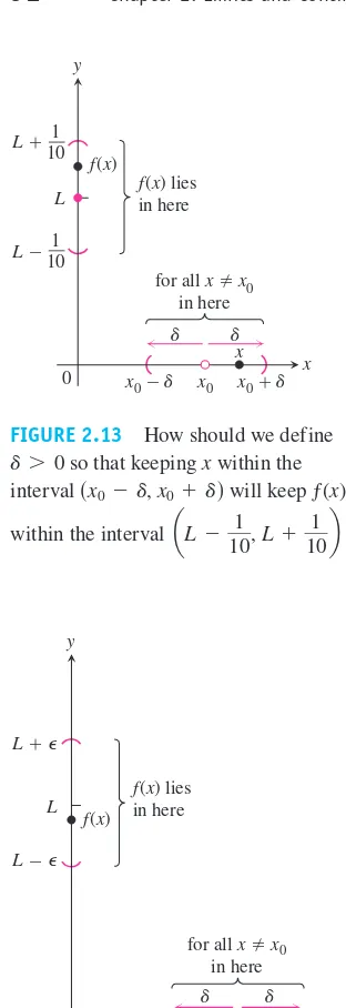
Suppose we are watching the values of a function ƒ(x) as xapproaches (without taking on the value of itself ). Certainly we want to be able to say that ƒ(x) stays within one-tenth of a unit of Las soon as xstays within some distance of (Figure 2.13). But that in itself is not enough, because as xcontinues on its course toward what is to prevent ƒ(x) from jit-tering about within the interval from to without tending toward L? We can be told that the error can be no more than or or . Each time, we find a new about so that keeping xwithin that interval satisfies the new error tolerance. And each time the possibility exists that ƒ(x) jitters away from Lat some stage.
The figures on the next page illustrate the problem. You can think of this as a quarrel between a skeptic and a scholar. The skeptic presents to prove that the limit does not exist or, more precisely, that there is room for doubt, and the scholar answers every challenge with a around
How do we stop this seemingly endless series of challenges and responses? By prov-ing that for every error tolerance that the challenger can produce, we can find, calculate, or conjure a matching distance that keeps x“close enough” to to keep ƒ(x) within that tolerance of L(Figure 2.14). This leads us to the precise definition of a limit.
x0
1>100,000 1>1000
92
Chapter 2: Limits and Continuity0
FIGURE 2.13 How should we define
so that keeping xwithin the
interval will keep ƒ(x)
FIGURE 2.14 The relation of and in
the definition of limit.
P
d
DEFINITION Limit of a Function
Let ƒ(x) be defined on an open interval about except possibly at itself. We say that the limit ofƒ(x) asxapproaches is the number L, and write
if, for every number there exists a corresponding number such that for all x,
One way to think about the definition is to suppose we are machining a generator shaft to a close tolerance. We may try for diameter L, but since nothing is perfect, we must be satisfied with a diameter ƒ(x) somewhere between and The is the measure of how accurate our control setting for xmust be to guarantee this degree of accu-racy in the diameter of the shaft. Notice that as the tolerance for error becomes stricter, we may have to adjust That is, the value of how tight our control setting must be, de-pends on the value of the error tolerance.
Examples: Testing the Definition
The formal definition of limit does not tell how to find the limit of a function, but it en-ables us to verify that a suspected limit is correct. The following examples show how the
definition can be used to verify limit statements for specific functions. (The first two ex-amples correspond to parts of Exex-amples 7 and 8 in Section 2.1.) However, the real purpose of the definition is not to do calculations like this, but rather to prove general theorems so that the calculation of specific limits can be simplified.
2.3 The Precise Definition of a Limit
93
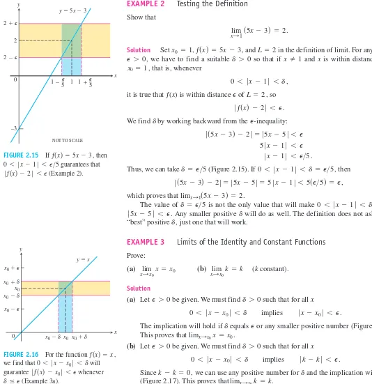
EXAMPLE 2 Testing the Definition Show that
Solution Set and in the definition of limit. For any given we have to find a suitable so that if and xis within distance of
that is, whenever
it is true that ƒ(x) is within distance of so
We find by working backward from the
Thus, we can take (Figure 2.15). If then
which proves that
The value of is not the only value that will make imply
Any smaller positive will do as well. The definition does not ask for a “best” positive just one that will work.
EXAMPLE 3 Limits of the Identity and Constant Functions
Prove:
(a) (b) (kconstant).
Solution
(a) Let be given. We must find such that for all x
The implication will hold if equals or any smaller positive number (Figure 2.16). This proves that
(b) Let be given. We must find such that for all x
Since we can use any positive number for and the implication will hold (Figure 2.17). This proves that
Finding Deltas Algebraically for Given Epsilons
In Examples 2 and 3, the interval of values about for which was less than was symmetric about x0and we could take to be half the length of that interval. Whend
P
94
Chapter 2: Limits and Continuityx
NOT TO SCALE
FIGURE 2.15 If then
guarantees that
FIGURE 2.16 For the function
such symmetry is absent, as it usually is, we can take to be the distance from to the in-terval’s nearerendpoint.
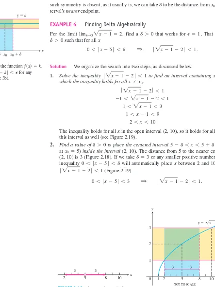
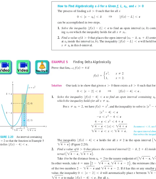
EXAMPLE 4 Finding Delta Algebraically
For the limit find a that works for That is, find a
such that for all x
Solution We organize the search into two steps, as discussed below.
1. Solve the inequality to find an interval containing on which the inequality holds for all
The inequality holds for all xin the open interval (2, 10), so it holds for all in this interval as well (see Figure 2.19).
2. Find a value of to place the centered interval (centered at ) inside the interval(2, 10). The distance from 5 to the nearer endpoint of (2, 10) is 3 (Figure 2.18). If we take or any smaller positive number, then the inequality will automatically place xbetween 2 and 10 to make
(Figure 2.19)
0 6 ƒx - 5ƒ 6 3 Q ƒ2x - 1 - 2ƒ 6 1 . ƒ2x - 1 - 2ƒ 6 1
0 6 ƒx - 5ƒ 6 d
d = 3 x0 = 5
5 - d 6 x 6 5 + d d 7 0
x Z 5 2 6 x 6 10
1 6 x - 1 6 9 1 6 2x - 1 6 3 -1 6 2x - 1 - 2 6 1
ƒ2x - 1 - 2ƒ 6 1 x Z x0.
x0 = 5 ƒ2x - 1 - 2ƒ 6 1
0 6 ƒx - 5ƒ 6 d Q ƒ2x - 1 - 2ƒ 6 1 . d 7 0
P = 1 . d 7 0
limx:52x - 1 = 2 ,
x0
d
2.3 The Precise Definition of a Limit
95
k⫺⑀
k⫹⑀
k
0 x0⫺␦ x0 x0⫹␦
x y
y ⫽ k
FIGURE 2.17 For the function
we find that for any
positive (Example d 3b). ƒƒsxd - kƒ 6 P
ƒsxd = k,
x 10
2 8
3
5 3
FIGURE 2.18 An open interval of
radius 3 about will lie inside the
open interval (2, 10). x0 = 5
x y
0 1 2 5 8 10
1 2 3
3 3
y⫽ 兹x⫺ 1
NOT TO SCALE
FIGURE 2.19 The function and intervals
EXAMPLE 5 Finding Delta Algebraically
Prove that if
Solution Our task is to show that given there exists a such that for all x
1. Solve the inequality to find an open interval containing on which the inequality holds for all
For we have and the inequality to solve is
The inequality holds for all in the open interval (Figure 2.20).
2. Find a value of that places the centered interval inside the
in-terval
Take to be the distance from to the nearer endpoint of
In other words, take the minimum(the smaller)
of the two numbers and If has this or any smaller positive value, the inequality will automatically place xbetween and
to make For all x,
This completes the proof.
0 6 ƒx - 2ƒ 6 d Q ƒƒsxd - 4ƒ 6 P. ƒƒsxd - 4ƒ 6 P.
24 + P
24 - P 0 6 ƒx - 2ƒ 6 d
d
24 + P - 2 . 2 - 24 - P
d = min
E
2 - 24 - P, 24 + P - 2F
,A
24 - P, 24 + PB
.x0 = 2
d
A
24 - P, 24 + PB
.s2 - d, 2 + dd d 7 0
24 + P
B
A
24 - P, x Z 2
ƒƒsxd - 4ƒ 6 P
24 - P 6 x 6 24 + P. 24 - P 6 ƒxƒ 6 24 + P
4 - P 6 x2 6 4 + P -P 6 x2 - 4 6 P
ƒx2 - 4ƒ 6 P
ƒx2 - 4ƒ 6 P: ƒsxd = x2,
x Z x0 = 2 ,
x Z x0.
x0 = 2 ƒƒsxd - 4ƒ 6 P
0 6 ƒx - 2ƒ 6 d Q ƒƒsxd - 4ƒ 6 P. d 7 0 P 7 0
ƒsxd = ex
2, x Z 2
1, x = 2.
limx:2 ƒsxd = 4
96
Chapter 2: Limits and ContinuityHow to Find Algebraically a for a Given f, L, and The process of finding a such that for all x
can be accomplished in two steps.
1. Solve the inequality to find an open interval (a,b) contain-ing on which the inequality holds for all
2. Find a value of that places the open interval centered at inside the interval (a,b). The inequality will hold for all
in this d-interval. x Z x0
ƒƒsxd - Lƒ 6 P x0
sx0 - d, x0 + dd
d 7 0
x Z x0.
x0
ƒƒsxd - Lƒ 6 P
0 6 ƒx - x0ƒ 6 d Q ƒƒsxd - Lƒ 6 P
d 7 0
P>0
x0, D
Assumes see P 6 4 ; below.
An open interval about that solves the inequality
x0 =2 0
4
4 ⫺ ⑀ 4 ⫹ ⑀
(2, 1) (2, 4)
2 x
y
兹4 ⫺ ⑀ 兹4 ⫹ ⑀
y ⫽ x2
FIGURE 2.20 An interval containing
so that the function in Example 5 satisfies ƒƒsxd - 4ƒ 6 P.
Why was it all right to assume Because, in finding a such that for all
implied we found a that would work for
any larger as well.
Finally, notice the freedom we gained in letting
We did not have to spend time deciding which, if either, number was the smaller of the two. We just let represent the smaller and went on to finish the argument.
Using the Definition to Prove Theorems
We do not usually rely on the formal definition of limit to verify specific limits such as those in the preceding examples. Rather we appeal to general theorems about limits, in particular the theorems of Section 2.2. The definition is used to prove these theorems (Appendix 2). As an example, we prove part 1 of Theorem 1, the Sum Rule.
EXAMPLE 6 Proving the Rule for the Limit of a Sum
Given that and prove that
Solution Let be given. We want to find a positive number such that for all x
Regrouping terms, we get
Since there exists a number such that for all x
Similarly, since there exists a number such that for all x
Let the smaller of and If then
so and so Therefore
This shows that
Let’s also prove Theorem 5 of Section 2.2.
EXAMPLE 7 Given that and and that
for all xin an open interval containing c(except possibly citself), prove that
Solution We use the method of proof by contradiction. Suppose, on the contrary, that Then by the limit of a difference property in Theorem 1,
Therefore, for any there exists such that
ƒsgsxd - ƒsxdd - sM - Ldƒ 6 P whenever 0 6 ƒx - cƒ 6 d. d 7 0
P 7 0 , lim
x:csgsxd - ƒsxdd = M - L. L 7 M.
L … M. ƒsxd … gsxd limx:c gsxd = M,
limx:c ƒsxd = L
limx:csƒsxd + gsxdd = L + M.
ƒƒsxd + gsxd - sL + Mdƒ 6 P 2 +
P 2 = P. ƒgsxd - Mƒ 6 P>2 . ƒx - cƒ 6 d2,
ƒƒsxd - Lƒ 6 P>2 ,
ƒx - cƒ 6 d1, 0 6 ƒx - cƒ 6 d
d2. d1 d = min 5d1, d26,
0 6 ƒx - cƒ 6 d2 Q ƒgsxd - Mƒ 6 P>2 . d2 7 0 limx:c gsxd = M,
0 6 ƒx - cƒ 6 d1 Q ƒƒsxd - Lƒ 6 P>2 . d1 7 0
limx:c ƒsxd = L,
… ƒƒsxd - Lƒ + ƒgsxd - Mƒ. ƒƒsxd + gsxd - sL + Mdƒ = ƒsƒsxd - Ld + sgsxd - Mdƒ
0 6 ƒx - cƒ 6 d Q ƒƒsxd + gsxd - sL + Mdƒ 6 P. d
P 7 0
lim x:csƒsxd
+ gsxdd = L + M. limx:c gsxd = M,
limx:c ƒsxd = L
d
24 + P - 2
F
.d = min
E
2 - 24 - P, Pd
ƒƒsxd - 4ƒ 6 P 6 4 , x, 0 6 ƒx - 2ƒ 6 d
d
P 6 4 ?
2.3 The Precise Definition of a Limit
97
Since by hypothesis, we take in particular and we have a number such that
Since for any number a, we have
which simplifies to
But this contradicts Thus the inequality must be false. Therefore L … M.
L 7 M ƒsxd … gsxd.
gsxd 6 ƒsxd whenever 0 6 ƒx - cƒ 6 d.
sgsxd - ƒsxdd - sM - Ld 6 L - M whenever 0 6 ƒx - cƒ 6 d a … ƒaƒ
ƒsgsxd - ƒsxdd - sM - Ldƒ 6 L - M whenever 0 6 ƒx - cƒ 6 d. d 7 0
P = L - M L - M 7 0
98
Chapter 2: Limits and ContinuityEXERCISES 2.3
Centering Intervals About a Point
In Exercises 1–6, sketch the interval (a, b) on the x-axis with the
point inside. Then find a value of such that for all
1.
Finding Deltas Graphically
In Exercises 7–14, use the graphs to find a such that for all x
7. 8.
NOT TO SCALE
–3
NOT TO SCALE
x0⫽ 5
NOT TO SCALE
L⫽ 4
NOT TO SCALE
y⫽x2
NOT TO SCALE
13. 14.
Finding Deltas Algebraically
Each of Exercises 15–30 gives a function ƒ(x) and numbers and In each case, find an open interval about on which the
in-equality holds. Then give a value for such
that for all x satisfying the inequality
holds.
NOT TO SCALE
2.5
More on Formal Limits
Each of Exercises 31–36 gives a function ƒ(x), a point , and a
posi-tive number Find Then find a number such
that for all x
Prove the limit statements in Exercises 37–50.
37. 38.
50.
Theory and Examples
51. Define what it means to say that
52. Prove that if and only if
53. A wrong statement about limits Show by example that the fol-lowing statement is wrong.
The number Lis the limit of ƒ(x) as xapproaches if ƒ(x) gets closer to Las xapproaches
Explain why the function in your example does not have the given value of Las a limit as
54. Another wrong statement about limits Show by example that the following statement is wrong.
The number Lis the limit of ƒ(x) as xapproaches if, given any there exists a value of xfor which
Explain why the function in your example does not have the given value of Las a limit as
55. Grinding engine cylinders Before contracting to grind engine cylinders to a cross-sectional area of you need to know how much deviation from the ideal cylinder diameter of
in. you can allow and still have the area come within of
the required To find out, you let and look for
the interval in which you must hold xto make What interval do you find?
56. Manufacturing electrical resistors Ohm’s law for electrical cir-cuits like the one shown in the accompanying figure states that In this equation, Vis a constant voltage, Iis the current in amperes, and Ris the resistance in ohms. Your firm has been asked to supply the resistors for a circuit in which Vwill be 120 V = RI.
We can prove that by providing an such that
no possible satisfies the condition
We accomplish this for our candidate by showing that for each
there exists a value of xsuch that
57.
100
Chapter 2: Limits and Continuitya. Let Show that no possible satisfies the following condition:
That is, for each show that there is a value of xsuch that
This will show that b. Show that
59. For the function graphed here, explain why a.
2.3 The Precise Definition of a Limit
101
60. a. For the function graphed here, show that
b. Does appear to exist? If so, what is the value of
the limit? If not, why not?
COMPUTER EXPLORATIONS
In Exercises 61–66, you will further explore finding deltas graphi-cally. Use a CAS to perform the following steps:
a. Plot the function near the point being approached.
b. Guess the value of the limit Land then evaluate the limit symbolically to see if you guessed correctly.
c. Using the value graph the banding lines
and together with the function ƒ near
d. From your graph in part (c), estimate a such that for all x
Test your estimate by plotting and over the interval
For your viewing window use
and If any
function values lie outside the interval your
choice of was too large. Try again with a smaller estimate.
e. Repeat parts (c) and (d) successively for and
102
Chapter 2: Limits and ContinuityOne-Sided Limits and Limits at Infinity
In this section we extend the limit concept to one-sided limits, which are limits as x ap-proaches the number from the left-hand side (where ) or the right-hand side only. We also analyze the graphs of certain rational functions as well as other functions with limit behavior as
One-Sided Limits
To have a limit Las xapproaches c, a function ƒ must be defined on both sidesof cand its values ƒ(x) must approach Las xapproaches cfrom either side. Because of this, ordinary limits are called two-sided.
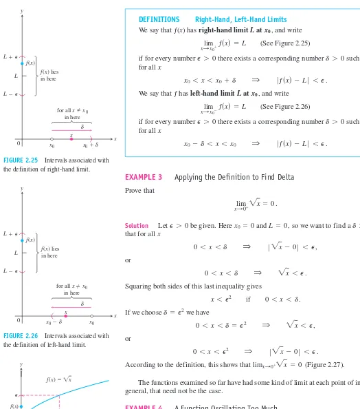
If ƒ fails to have a two-sided limit at c, it may still have a one-sided limit, that is, a limit if the approach is only from one side. If the approach is from the right, the limit is a
right-hand limit. From the left, it is a left-hand limit.
The function (Figure 2.21) has limit 1 as xapproaches 0 from the right, and limit as xapproaches 0 from the left. Since these one-sided limit values are not the same, there is no single number that ƒ(x) approaches as xapproaches 0. So ƒ(x) does not have a (two-sided) limit at 0.
Intuitively, if ƒ(x) is defined on an interval (c,b), where and approaches arbi-trarily close to Las xapproaches cfrom within that interval, then ƒ has right-hand limitL at c. We write
The symbol means that we consider only values of xgreater than c.
Similarly, if ƒ(x) is defined on an interval (a,c), where and approaches arbi-trarily close to Mas xapproaches cfrom within that interval, then ƒ has left-hand limitM at c. We write
The symbol means that we consider only xvalues less than c. These informal definitions are illustrated in Figure 2.22. For the function in Figure 2.21 we have
lim
x:0+ ƒsxd = 1 and xlim:0- ƒsxd = -1 .
ƒsxd = x>ƒxƒ “x:c-”
lim
x:c- ƒsxd = M.
a 6 c “x:c+”
lim
x:c+ ƒsxd = L.
c 6 b, -1
ƒsxd = x>ƒxƒ
x:; q. sx 7 x0d
x 6 x0
x0
2.4
x y
1
0
–1
y⫽ x 兩x兩
FIGURE 2.21 Different right-hand and
left-hand limits at the origin.
x y
0 x
y
c x x c
L f(x)
0
M f(x)
lim f(x) ⫽L
x→c⫹ (b) lim f(x) ⫽M
(a)
x→c⫺
FIGURE 2.22 (a) Right-hand limit as xapproaches c. (b) Left-hand limit as x