An Introduction to Machine Learning 2nd Edition pdf pdf

(1)

Miroslav Kubat

An Introduction

to Machine

(2)

(3)

An Introduction to Machine

Learning

Second Edition

(4)

Miroslav Kubat

Department of Electrical and Computer Engineering University of Miami

Coral Gables, FL, USA

ISBN 978-3-319-63912-3 ISBN 978-3-319-63913-0 (eBook) DOI 10.1007/978-3-319-63913-0

Library of Congress Control Number: 2017949183

This work is subject to copyright. All rights are reserved by the Publisher, whether the whole or part of the material is concerned, specifically the rights of translation, reprinting, reuse of illustrations, recitation, broadcasting, reproduction on microfilms or in any other physical way, and transmission or information storage and retrieval, electronic adaptation, computer software, or by similar or dissimilar methodology now known or hereafter developed.

The use of general descriptive names, registered names, trademarks, service marks, etc. in this publication does not imply, even in the absence of a specific statement, that such names are exempt from the relevant protective laws and regulations and therefore free for general use.

The publisher, the authors and the editors are safe to assume that the advice and information in this book are believed to be true and accurate at the date of publication. Neither the publisher nor the authors or the editors give a warranty, express or implied, with respect to the material contained herein or for any errors or omissions that may have been made. The publisher remains neutral with regard to jurisdictional claims in published maps and institutional affiliations.

Printed on acid-free paper

This Springer imprint is published by Springer Nature The registered company is Springer International Publishing AG

(5)

(6)

Introduction

Machine learning has come of age. And just in case you might think this is a mere platitude, let me clarify.

The dream that machines would one day be able to learn is as old as computers themselves, perhaps older still. For a long time, however, it remained just that: a dream. True, Rosenblatt’s perceptron did trigger a wave of activity, but in retrospect, the excitement has to be deemed short-lived. As for the attempts that followed, these fared even worse; barely noticed, often ignored, they never made a breakthrough— no software companies, no major follow-up research, and not much support from funding agencies. Machine learning remained an underdog, condemned to live in the shadow of more successful disciplines. The grand ambition lay dormant.

And then it all changed.

A group of visionaries pointed out a weak spot in the knowledge-based systems that were all the rage in the 1970s’ artificial intelligence: where was the “know-ledge” to come from? The prevailing wisdom of the day insisted that it should take the form ofif-thenrules put together by the joint effort of engineers and field experts. Practical experience, though, was unconvincing. Experts found it difficult to communicate what they knew to engineers. Engineers, in turn, were at a loss as to what questions to ask and what to make of the answers. A few widely publicized success stories notwithstanding, most attempts to create a knowledge base of, say, tens of thousands of such rules proved frustrating.

The proposition made by the visionaries was both simple and audacious. If it is so hard to tell a machine exactly how to go about a certain problem, why not provide the instruction indirectly, conveying the necessary skills by way of examples from which the computer will—yes—learn!

Of course, this only makes sense if we can rely on the existence of algorithms to do the learning. This was the main difficulty. As it turned out, neither Rosenblatt’s perceptron nor the techniques developed after it were very useful. But the absence of the requisite machine-learning techniques was not an obstacle; rather, it was a challenge that inspired quite a few brilliant minds. The idea of endowing computers with learning skills opened new horizons and created a large amount of excitement. The world was beginning to take notice.

(11)

The bombshell exploded in 1983.Machine Learning: The AI Approach1 was a thick volume of research papers which proposed the most diverse ways of addressing the great mystery. Under their influence, a new scientific discipline was born—virtually overnight. Three years later, a follow-up book appeared and then another. A soon-to-become-prestigious scientific journal was founded. Annual conferences of great repute were launched. And dozens, perhaps hundreds, of doctoral dissertations, were submitted and successfully defended.

In this early stage, the question was not onlyhowto learn but alsowhatto learn andwhy. In retrospect, those were wonderful times, so creative that they deserve to be remembered with nostalgia. It is only to be regretted that so many great thoughts later came to be abandoned. Practical needs of realistic applications got the upper hand, pointing to the most promising avenues for further efforts. After a period of enchantment, concrete research strands crystallized: induction of theif-thenrules for knowledge-based systems; induction of classifiers, programs capable of improving their skills based on experience; automatic fine-tuning of Prolog programs; and some others. So many were the directions that some leading personalities felt it necessary to try to steer further development by writing monographs, some successful, others less so.

An important watershed was Tom Mitchell’s legendary textbook.2_This summa-rized the state of the art of the field in a format appropriate for doctoral students and scientists alike. One by one, universities started offering graduate courses that were usually built around this book. Meanwhile, the research methodology became more systematic, too. A rich repository of machine-leaning test beds was created, making it possible to compare the performance or learning algorithms. Statistical methods of evaluation became widespread. Public domain versions of most popular programs were made available. The number of scientists dealing with this discipline grew to thousands, perhaps even more.

Now, we have reached the stage where a great many universities are offering machine learning as an undergraduate class. This is quite a new situation. As a rule, these classes call for a different kind of textbook. Apart from mastering the baseline techniques, future engineers need to develop a good grasp of the strengths and weaknesses of alternative approaches; they should be aware of the peculiarities and idiosyncrasies of different paradigms. Above all, they must understand the circumstances under which some techniques succeed and others fail. Only then will they be able to make the right choices when addressing concrete applications. A textbook that is to provide all of the above should contain less mathematics, but a lot of practical advice.

These then are the considerations that have dictated the size, structure, and style of a teaching text meant to provide the material for a one-semester introductory course.

(12)

Introduction xiii

The first problem is the choice of material. At a time when high-tech companies are establishing machine-learning groups, universities have to provide the students with such knowledge, skills, and understanding that are relevant to the current needs of the industry. For this reason, preference has been given to Bayesian classifiers, nearest-neighbor classifiers, linear and polynomial classifiers, decision trees, the fundamentals of the neural networks, and the principle of the boosting algorithms. Significant space has been devoted to certain typical aspects of concrete engineering applications. When applied to really difficult tasks, the baseline techniques are known to behave not exactly the same way they do in the toy domains employed by the instructor. One has to know what to expect.

The book consists of 17 chapters, each covering one major topic. The chapters are divided into sections, each devoted to one critical problem. The student is advised to proceed to the next section only after having answered the set of 2–4 “control questions” at the end of the previous section. These questions are here to help the student decide whether he or she has mastered the given material. If not, it is necessary to return to the previous text.

(13)

A Simple Machine-Learning Task

You will find it difficult to describe your mother’s face accurately enough for your friend to recognize her in a supermarket. But if you show him a few of her photos, he will immediately spot the tell-tale traits he needs. As they say, a picture—an example—is worth a thousand words.

This is what we want our technology to emulate. Unable to define certain objects or concepts with adequate accuracy, we want to convey them to the machine by way of examples. For this to work, however, the computer has to be able to convert the examples into knowledge. Hence our interest in algorithms and techniques for

machine learning, the topic of this textbook.

The first chapter formulates the task as a search problem, introducing hill-climbing search not only as our preliminary attempt to address the machine-learning task, but also as a tool that will come handy in a few auxiliary problems to be encountered in later chapters. Having thus established the foundation, we will proceed to such issues as performance criteria, experimental methodology, and certain aspects that make the learning process difficult—and interesting.

1.1 Training Sets and Classifiers

Let us introduce the problem, and certain fundamental concepts that will accompany us throughout the rest of the book.

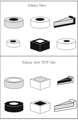
The Set of Pre-Classified Training Examples Figure 1.1 shows six pies that

Johnny likes, and six that he does not. Thesepositiveandnegative examplesof the underlying concept constitute atraining setfrom which the machine is to induce a

classifier—an algorithm capable of categorizing any future pie into one of the two

classes: positive and negative.

(14)

2 1 A Simple Machine-Learning Task

Johnny likes:

Johnny does NOT like:

Fig. 1.1 A simple machine-learning task: induce a classifier capable of labeling future pies as positive and negative instances of “a pie that Johnny likes”

The number of classes can of course be greater. Thus a classifier that decides

whether a landscape snapshot was taken in spring, summer, fall, or

winter distinguishes four. Software that identifies characters scribbled on an

(15)

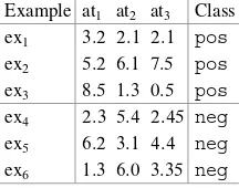
Table 1.1 The twelve training examples expressed in a matrix form

Crust Filling

Example Shape Size Shade Size Shade Class

ex1 Circle Thick Gray Thick Dark pos

ex2 Circle Thick White Thick Dark pos

ex3 Triangle Thick Dark Thick Gray pos

ex4 Circle Thin White Thin Dark pos

ex5 Square Thick Dark Thin White pos

ex6 Circle Thick White Thin Dark pos

ex7 Circle Thick Gray Thick White neg

ex8 Square Thick White Thick Gray neg

ex9 Triangle Thin Gray Thin Dark neg

ex10 Circle Thick Dark Thick White neg

ex11 Square Thick White Thick Dark neg

ex12 Triangle Thick White Thick Gray neg

Attribute Vectors To be able to communicate the training examples to the

machine, we have to describe them in an appropriate way. The most common mechanism relies on so-called attributes. In the “pies” domain, five may be suggested: shape (circle, triangle, and square), crust-size (thin or thick),

crust-shade (white, gray, or dark), filling-size (thin or thick), and

filling-shade(white, gray, or dark). Table 1.1specifies the values of these attributes for the twelve examples in Fig.1.1. For instance, the pie in the upper-left corner of the picture (the table calls it ex1) is described by the following conjunction:

(shape=circle) AND (crust-size=thick) AND (crust-shade=gray) AND (filling-size=thick) AND (filling-shade=dark)

A Classifier to Be Induced The training set constitutes the input from which we

are to induce the classifier. Butwhatclassifier?

Suppose we want it in the form of a boolean function that is true for positive examples and false for negative ones. Checking the expression

[(shape=circle) AND (filling-shade=dark)] against the training set, we can see that its value isfalsefor all negative examples: while itispossible to find negative examples that are circular, none of these has a dark filling. As for the positive examples, however, the expression istruefor four of them andfalsefor the remaining two. This means that the classifier makes two errors, a transgression we might refuse to tolerate, suspecting there is a better solution. Indeed, the reader will easily verify that the following expression never goes wrong on the entire training set:

(16)

Problems with a Brute-Force Approach How does a machine find a classifier of

this kind? Brute force (something that computers are so good at) will not do here. Just consider how many different examples can be distinguished by the given set of attributes in the “pies” domain. For each of the three differentshapes, there are two alternativecrust-sizes, the number of combinations being32_D6. For each of these, the next attribute,crust-shade, can acquire three different values, which brings the number of combinations to323_D18. Extending this line of reasoning toallattributes, we realize that the size of theinstance spaceis

32323_D108different examples.

Each subset of these examples—and there are2108_{subsets!—may constitute the} list of positive examples of someone’s notion of a “good pie.” And each such subset can be characterized by at least one boolean expression. Running each of these classifiers through the training set is clearly out of the question.

Manual Approach and Search Uncertain about how to invent a

classifier-inducing algorithm, we may try to glean some inspiration from an attempt to create a classifier “manually,” by the good old-fashioned pencil-and-paper method. When doing so, we begin with some tentative initial version, say,

shape=circular. Having checked it against the training set, we find it to be true for four positive examples, but also for two negative ones. Apparently, the classifier needs to be “narrowed” (specialized) so as to exclude the two negative examples. One way to go about the specialization is to add a conjunction,

such as when turning shape=circular into [(shape=circular) AND

(filling-shade=dark)]. This new expression, while falsefor all negative examples, is still imperfect because it covers only four (ex1, ex2, ex4, and

ex6) of the six positive examples. The next step should therefore attempt some generalization, perhaps by adding a disjunction:{[(shape=circular) AND (filling-shade=dark)] OR (crust-size=thick)}. We continue in this way until we find a 100% accurate classifier (if it exists).

The lesson from this little introspection is that the classifier can be created by means of a sequence of specialization and generalization steps which gradually modify a given version of the classifier until it satisfies certain predefined require-ments. This is encouraging. Readers with background in Artificial Intelligence will recognize this procedure as asearchthrough the space of boolean expressions. And Artificial Intelligence is known to have developed and explored quite a few of search algorithms. It may be an idea to take a look at least at one of them.

What Have You Learned?

To make sure you understand the topic, try to answer the following questions. If needed, return to the appropriate place in the text.

• What is the input and output of the learning problem we have just described? • How do we describe the training examples? What is instance space? Can we

(17)

• In the “pies” domain, find a boolean expression that correctly classifies all the training examples from Table1.1.

1.2 Minor Digression: Hill-Climbing Search

Let us now formalize what we mean by search, and then introduce one pop-ular algorithm, the so-called hill climbing. Artificial Intelligence defines search

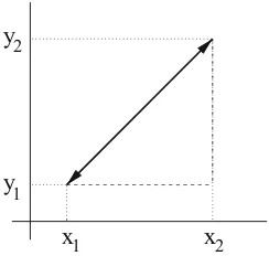
something like this: starting from aninitial state, find a sequence of steps which, proceeding through a set of interimsearch states, lead to a predefinedfinal state. The individual steps—transitions from one search state to another—are carried out

bysearch operatorswhich, too, have been pre-specified by the programmer. The

order in which the search operators are applied follows a specificsearch strategy

(Fig.1.2).

Hill Climbing: An Illustration One popular search strategy ishill climbing. Let

us illustrate its essence on a well-known brain-teaser, the sliding-tiles puzzle. The board of a trivial version of this game consists of nine squares arranged in three rows, eight covered by numbered tiles (integers from 1 to 8), the last left empty. We convert one search state into another by sliding to the empty square a tile from one of its neighbors. The goal is to achieve a pre-specified arrangement of the tiles.

Search Operators Search Strategy

Final State Initial State

Search Agent

(18)

The flowchart in Fig.1.3 starts with a concrete initial state, in which we can choose between two operators: “move tile-6 up” and “move tile-2 to the left.” The choice is guided by anevaluation functionthat estimates for each state its distance from the goal. A simple possibility is to count the squares that the tiles have to traverse before reaching their final destinations. In the initial state, tiles 2, 4, and 5 are already in the right locations; tile 3 has to be moved by four squares; and each of the tiles 1, 6, 7, and 8 have to be moved by two squares. This sums up to distanced_D4_C42_D12.

In Fig.1.3, each of the two operators applicable to the initial state leads to a state whose distance from the final state isd _D 13. In the absence of any other guidance, we choose randomly and go to the left, reaching the situation where the empty square is in the middle of the top row. Here, three moves are possible. One of them would only get us back to the initial state, and can thus be ignored; as for the remaining two, one results in a state withd _D14, the other in a state withd_D 12. The latter being the lower value, this is where we go. The next step is trivial because only one move gets us to a state that has not been visited before. After this, we again face the choice between two alternatives . . . and this how the search continues until it reaches the final state.

Alternative Termination Criteria and Evaluation Functions Othertermination

criteria can be considered, too. The search can be instructed to stop when the

maximum allotted time has elapsed (we do not want the computer to run forever), when the number of visited states has exceeded a certain limit, when something sufficiently close to the final state has been found, when we have realized that all states have already been visited, and so on, the concrete formulation reflecting critical aspects of the given application, sometimes combining two or more criteria in one.

By the way, the evaluation function employed in the sliding-tiles example was fairly simple, barely accomplishing its mission: to let the user convey some notion of his or her understanding of the problem, to provide a hint as to which move a human solver might prefer. To succeed in a realistic application, we would have to come up with a more sophisticated function. Quite often,manydifferent alternatives can be devised, each engendering a different sequence of steps. Some will be quick in reaching the solution, others will follow a more circuitous path. The program’s performance will then depend on the programmer’s ability to pick the right one.

The Algorithm of Hill Combing The algorithm is summarized by the pseudocode

(19)

Final State:

Fig. 1.3 Hill climbing. Circled integers indicate the order in which the search states are visited. dis a state’s distance from the final state as calculated by the given evaluation function. Ties are broken randomly

state, and a fifth sorts the “child” states according to the distances thus calculated and places them at the front of the listL. And the last function checks if a termination criterion has been satisfied.1

One last observation: at some of the states in Fig.1.3, no “child” offers any improvement over its “parent,” a lowerd-value being achieved only after temporary compromises. This is what a mountain climber may experience, too: sometimes, he has to traverse a valley before being able to resume the ascent. The mountain-climbing metaphor, by the way, is what gave this technique its name.

1_{For simplicity, the pseudocode ignores termination criteria other than reaching, or failing to reach,}

(20)

Table 1.2 Hill-climbing search algorithm

1. Create two lists,LandLseen. At the beginning,Lcontains only the initial state, andLseenis empty.

2. Letnbe the first element ofL. Compare this state with the final state. If they are identical, stop with success.

3. Apply tonall available search operators, thus obtaining a set of new states. Discard those states that already exist inLseen. As for the rest, sort them by the evaluation function and place them at the front ofL.

4. TransfernfromLinto the list,Lseen, of the states that have been investigated. 5. IfL_{D ;}, stop and report failure. Otherwise, go to 2.

What Have You Learned?

• How does Artificial Intelligence define the search problem? What do we understand under the terms, “search space” and “search operators”?

• What is the role of the evaluation function? How does it affect the hill-climbing behavior?

1.3 Hill Climbing in Machine Learning

We are ready to explore the concrete ways of applying hill climbing to the needs of machine learning.

Hill Climbing and Johnny’s Pies Let us begin with the problem of how to decide

which pies Johnny likes. The input consists of a set of training examples, each described by the available attributes. The output—the final state—is a boolean expression that istruefor each positive example in the training set, andfalsefor each negative example. The expression involves attribute-value pairs, logical operators (conjunction, disjunction, and negation), and such combination of parentheses as may be needed. The evaluation function measures the given expression’s error rate on the training set. For theinitial state, any randomly generated expression can be used. In Fig.1.4, we chose(shape=circle), on the grounds that more than a half of the training examples are circular.

As for the search operator, one possibility is to add a conjunction as illustrated in the upper part of Fig.1.4: for instance, the root’s leftmost child

is obtained by replacing (shape=circle) with [(shape=circle) AND

(21)

shape = circle shape = triangle fill size = thin

1

2

3 ( shape = circle fill shade = dark )

(shape = circle ( shape = circle

Fig. 1.4 Hill-climbing search in the “pies” domain

“ANDed.” Since the remaining four attributes (apart fromshape) acquire 2, 3, 2, and 3 different values, respectively, the total number of terms that can be added to

(shape=circle)is223_D36.2

Alternatively, we may choose to add a disjunction, as illustrated (in the picture) by the three expansions of the leftmost child. Other operators may “remove a conjunct,” “remove a disjunct,” “add a negation,” “negate a term,” various ways of manipulating parentheses, and so on. All in all, hundreds of search operators can be applied to each state, and then again to the resulting states. This can be hard to manage even in this very simple domain.

Numeric Attributes In the “pies” domain, each attribute acquires one out of a

few discrete values, but in realistic applications, some attributes will probably be numeric. For instance, each pie has aprice, an attribute whose values come from a continuous domain. What will the search look like then?

To keep things simple, suppose there are only two attributes: weight and

price. This limitation makes it possible, in Fig.1.5, to represent each training example by a point in a plane. The reader can see that examples belonging to the same class tend to occupy a specific region, and curves separating individual regions can be defined—expressed mathematically as lines, circles, polynomials. For instance, the right part of Fig.1.5shows three different circles, each of which can act as a classifier: examples inside the circle are deemed positive; those outside, negative. Again, some of these classifiers are better than others. How will hill climbing go about finding the best ones? Here is one possibility.

(22)

Price

Weight ($3, 1.2lb)

Price

Weight ($3, 1.2lb)

Fig. 1.5 On the left: a domain with continuous attributes;on the right: some “circular” classifiers

Hill Climbing in a Domain with Numeric Attributes

Initial State A circle is defined by its center and radius. We can identify the initial center with a randomly selected positive example, making the initial radius so small that the circle contains only this single example.

Search Operators Two search operators can be used: one increases the circle’s

radius, and the other shifts the center from one training example to another. In the former, we also have to determinehow muchthe radius should change. One idea is to increase it only so much as to make the circle encompass one additional training example. At the beginning, only one training example is inside. After the first step, there will be two, then three, four, and so on.

Final State The circle may not be an ideal figure to represent the positive region. In this event, a 100% accuracy may not be achievable, and we may prefer to define the final state as, say, a “classifier that correctly classifies 95% of the training examples.”

Evaluation Function As before, we choose to minimize the error rate.

What Have You Learned?

• What aspects of search must be specified before we can employ hill climbing in machine learning?

(23)

1.4 The Induced Classifier’s Performance

So far, we have measured the error rate by comparing the training examples’ known classes with those recommended by the classifier. Practically speaking, though, our goal isnotto re-classify objects whose classes we already know; what we really want is to labelfuture examples, those of whose classes we are as yet ignorant. The classifier’s anticipated performance on these is estimated experimentally. It is important to know how.

Independent Testing Examples The simplest scenario will divide the available

pre-classified examples into two parts: the training set, from which the classifier is induced, and thetesting set, on which it is evaluated (Fig.1.6). Thus in the “pies” domain, with its 12 pre-classified examples, the induction may be carried out on randomly selected eight, and the testing on the remaining four. If the classifier then “guesses” correctly the class of three testing examples (while going wrong on one), its performance is estimated as 75%.

Reasonable though this approach may appear, it suffers from a major drawback: a random choice of eight training examples may not be sufficiently representative of the underlying concept—and the same applies to the (even smaller) testing set. If we induce the meaning of amammalfrom a training set consisting of a whale, a dolphin, and a platypus, the learner may be led to believe that mammals live in the sea (whale, dolphin), and sometimes lay eggs (platypus), hardly an opinion a biologist will embrace. And yet, another choice of trainingexamples may result in a

Fig. 1.6 Pre-classified examples are divided into the training and testing sets

set

training testing set

available examples

classifier satisfying the highest standards. The point is, a different training/testing set division gives rise to a different classifier—and also to a different estimate of future performance. This is particularly serious if the number of pre-classified examples is small.

Suppose we want to compare two machine learning algorithms in terms of the quality of the products they induce. The problem of non-representative training sets can be mitigated by so-calledrandom subsampling.3_{The idea is to repeat the} random division into the training and testing sets several times, always inducing a classifier from thei-th training set, and then measuring the error rate,Ei, on thei-th

testing set. The algorithm that delivers classifiers with the lower average value of

Ei’s is deemed better—as far as classification performance is concerned.

(24)

The Need for Explanations In some applications, establishing the class of each

example is not enough. Just as desirable is to know the reasons behind the classification. Thus a patient is unlikely to give consent to amputation if the only argument in support of surgery is, “this is what our computer says.” But how to find a better explanation?

In the “pies” domain, a lot can be gleaned from the boolean expression itself. For instance, we may notice that a pie was labeled as negative whenever its shape was square, and its filling white. Combining this observation with alternative sources of knowledge may offer useful insights: the dark shade of the filling may indicate poppy, an ingredient Johnny is known to love; or the crust of circular pies turns out to be more crispy than that of square ones; and so on. The knowledge obtained in this manner can be more desirable than the classification itself.

By contrast, the classifier in the “circles” domain is a mathematical expression that acts as a “black box” which accepts an example’s description and returns the class label without telling us anything else. This is not necessarily a shortcoming. In some applications, an explanation is nothing more than a welcome bonus; in others, it is superfluous. Consider a classifier that accepts a digital image of a hand-written character and returns the letter it represents. The user who expects several pages of text to be converted into a Word document will hardly insist on a detailed explanation for each single character.

Existence of Alternative Solutions By the way, we should notice that many

apparently perfect classifiers can be induced from the given data. In the “pies” domain, the training set contained 12 examples, and the classes of the remaining 96 examples were unknown. Using some simple combinatorics, we realize that there are296_{classifiers that label correctly all training examples but differ in the way they} label the unknown 96. One induced classifier may label correctly every single future example—and another will misclassify them all.

What Have You Learned?

• How can we estimate the error rate on examples that have not been seen during learning?

• Why is error rate usually higher on the testing set than on the training set? • Give an example of a domain where the classifier also has to explain its action,

and an example of a domain where this is unnecessary.

(25)

1.5 Some Difficulties with Available Data

In some applications, the training set is created manually: an expert prepares the examples, tags them with class labels, chooses the attributes, and specifies the value of each attribute in each example. In other domains, the process is computerized. For instance, a company may want to be able to anticipate an employee’s intention to leave. Their database contains, for each person, the address, gender, marital status, function, salary raises, promotions—as well as the information about whether the person is still with the company or, if not, the day they left. From this, a program can obtain the attribute vectors, labeled as positive if the given person left within a year since the last update of the database record.

Sometimes, the attribute vectors are automatically extracted from a database, and labeled by an expert. Alternatively, some examples can be obtained from a database, and others added manually. Often, two or more databases are combined. The number of such variations is virtually unlimited.

But whatever the source of the examples, they are likely to suffer from imperfec-tions whose essence and consequences the engineer has to understand.

Irrelevant Attributes To begin with, some attributes are important, while others

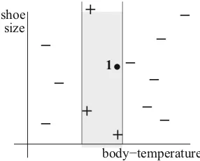
are not. While Johnny may be truly fond of poppy filling, his preference for a pie will hardly be driven by the cook’s shoe size. This is something to be concerned about:irrelevant attributes add to computational costs; they can even mislead the learner. Can they be avoided?

Usually not. True, in manually created domains, the expert is supposed to know which attributes really matter, but even here, things are not so simple. Thus the author of the “pies” domain might have done her best to choose those attributes she believed to matter. But unsure about the real reasons behind Johnny’s tastes, she may have included attributes whose necessity she suspected—but could not guarantee. Even more often the problems with relevance occur when the examples are extracted from a database. Databases are developed primarily with the intention to provide access to lots of information—of which usually only a tiny part pertains to the learning task. As to which part this is, we usually have no idea.

Missing Attributes Conversely, some critical attributes can be missing. Mindful of

his parents’ finances, Johnny may be prejudiced against expensive pies. The absence of attributepricewill then make it impossible to induce a good classifier: two examples, identical in terms of the available attributes, can differ in the values of the vital “missing” attribute. No wonder that, though identically described, one example is positive, and the other is negative. When this happens, we say that the training set isinconsistent. The situation is sometimes difficult to avoid: not only may the expert be ignorant of the relevance of attributeprice; it may be impossible to provide this attribute’s values, and the attribute thus cannot be used anyway.

Redundant Attributes Somewhat less damaging are attributes that areredundant

(26)

because it can be calculated by subtractingdate-of-birthfrom today’s date. Fortunately, redundant attributes are less dangerous than irrelevant or missing ones.

Missing Attribute Values In some applications, the user has no problems

identi-fying the right choice of attributes. The problem is, however, that the value of some attributes are not known. For instance, the company analyzing the database of its employees may not know, for each person, the number of children.

Attribute: Value Noise Attribute values and class labels often cannot be trusted on

account of unreliable sources of information, poor measurement devices, typos, the user’s confusion, and many other reasons. We say that the data suffer from various kinds ofnoise.

Stochastic noiseis random. For instance, since our body-weight varies during the day, the reading we get in the morning is different from the one in the evening. A human error can also play a part: lacking the time to take a patient’s blood pressure, a negligent nurse simply scribbles down a modification of the previous reading. By contrast,systematic noisedrags all values in the same direction. For instance, a poorly calibrated thermometer always gives a lower reading than it should. And something different occurs in the case ofarbitrary artifacts; here, the given value bears no relation to reality such as when an EEG electrode gets loose and, from that moment on, all subsequent readings will be zero.

Class-Label Noise Class labels suffer from similar problems as attributes. The

labels recommended by an expert may not have been properly recorded; alter-natively, some examples find themselves in a “gray area” between two classes, in which event the correct labels are not certain. Both cases represent stochastic noise, of which the latter may affect negatively only examples from the borderline region between the two classes. However, class-label noise can also be systematic: a physician may be reluctant to diagnose a rare disease unless the evidence is overwhelming—his class labels are then more likely to be negative than positive. Finally, arbitrary artifacts in class labels are encountered in domains where the classes are supplied by an automated process that has gone wrong.

Class-label noise can be more dangerous than attribute-value noise. Thus in the “circles” domain, an example located deep inside the positive region will stay there even if an attribute’s value is slightly modified; only the borderline example will suffer from being “sent across the border.” By contrast, class-label noise will invalidateanyexample.

What Have You Learned?

(27)

Learning:

Application:

Training

Concept _Examples Classifier

Classifier Example Concept_Label

Fig. 1.7 The training examples are used to induce a classifier. The classifier is then employed to classify future examples

• What is meant by “inconsistent training set”? What can be the cause? How can it affect the learning process?

• What kinds of noise do we know? What are their possible sources?

1.6 Summary and Historical Remarks

• Induction from a training set of pre-classified examples is the most deeply studied machine-learning task.

• Historically, the task is cast as search. One can propose a mechanism that exploits the well-established search technique of hill climbing defined by an initial state, final state, interim states, search operators, and evaluation functions.

• Mechanical use of search is not the ultimate solution, though. The rest of the book will explore more useful techniques.

• Classifier performance is estimated with the help of pre-classified testing data. The simplest performance criterion is error rate, the percentage of examples misclassified by the classifier. The baseline scenario is shown in Fig.1.7. • Two classifiers that both correctly classify all training examples may differ

significantly in their handling of the testing set.

• Apart from low error rate, some applications require that the classifier provides the reasons behind the classification.

• The quality of the induced classifier depends on training examples. The quality of the training examples depends not only on their choice, but also on the attributes used to describe them. Some attributes are relevant, others irrelevant or redundant. Quite often, critical attributes are missing.

(28)

Historical Remarks The idea of casting the machine-learning task as search was

popular in the 1980s and 1990s. While several “founding fathers” came to see things this way independently of each other, Mitchell [67] is often credited with being the first to promote the search-based approach; just as influential, however, was the family of AQ-algorithms proposed by Michalski [59]. The discipline got a major boost by the collection of papers edited by Michalski et al. [61]. They framed the mindset of a whole generation.

There is much more to search algorithms. The interested reader is referred to textbooks of Artificial Intelligence, of which perhaps the most comprehensive is Russell and Norvig [84] or Coppin [17].

The reader may find it interesting that the question of proper representation of concepts or classes intrigued philosophers for centuries. Thus John Stuart Mill [65] explored concepts that are related towhat the next chapter callsprobabilistic

a

l m

b c d

e f g h i j k

0.1

2.5 1.4 2.3

2.1 0.3

2.0 0.2 2.0 1.0 3.2

1.5 3.5

Fig. 1.8 Determine the order in which these search states are visited by heuristic search algorithms. The numbers next to the “boxes” give the values of the evaluation function for the individual search states

representation; and William Whewel [96] advocated prototypical representations that are close to the subject of our Chap.3.

1.7 Solidify Your Knowledge

(29)

Exercises

1. In the sliding-tiles puzzle, suggest a better evaluation function than the one used in the text.

2. Figure1.8shows a search tree where each node represents one search state and is tagged with the value of the evaluation function. In what order will these states be visited by hill-climbing search?

3. Suppose the evaluation function in the “pies” domain calculates the percentage of correctly classified training examples. Let the initial state be the expression describing the second positive example in Table 1.1. Hand-simulate the hill-climbing search that uses generalization and specialization operators.

4. What is the size of the instance space in a domain where examples are described by ten boolean attributes? How large is then the space of classifiers?

Give It Some Thought

1. In the “pies” domain, the size of the space of all classifiers is2108_{, provided that} each subset of the instance space can be represented by a distinct classifier. How much will the search space shrink if we permit only classifiers in the form of conjunctions of attribute-value pairs?

2. What kind of noise can you think of in the “pies” domain? What can be the source of this noise? What other issues may render training sets of this kind less than perfect?

3. Some classifiers behave as black boxes that do not offer much in the way of explanations. This, for instance, was the case of the “circles” domain. Suggest examples of domains where black-box classifiers are impractical, and suggest domains where this limitation does not matter.

4. Consider the data-related difficulties summarized in Sect.1.5. Which of them are really serious, and which can perhaps be tolerated?

5. What is the difference between redundant attributes and irrelevant attributes? 6. Take a class that you think is difficult to describe—for instance, the recognition

(30)

Computer Assignments

1. Write a program implementing hill climbing and apply it to the sliding-tiles puzzle. Choose appropriate representation for the search states, write a module that decides whether a state is a final state, and implement the search operators. Define two or three alternative evaluation functions and observe how each of them leads to a different sequence of search steps.

2. Write a program that will implement the “growing circles” algorithm from Sect.1.3. Create a training set of two-dimensional examples such as those in Fig.1.5. The learning program will use the hill-climbing search. The evaluation function will calculate the percentage of training examples correctly classified by the classifier. Consider the following search operators: (1) increase/decrease the radius of the circle, (2) use a different training example as the circle’s center. 3. Write a program that will implement the search for the description of the “pies

(31)

Probabilities: Bayesian Classifiers

The earliest attempts to predict an example’s class based on the known attribute values go back to well before World War II—prehistory, by the standards of computer science. Of course, nobody used the term “machine learning,” in those days, but the goal was essentially the same as the one addressed in this book.

Here is the essence of the solution strategy they used: using the Bayesian probabilistic theory, calculate for each class the probability of the given object belonging to it, and then choose the class with the highest value.

2.1 The Single-Attribute Case

Let us start with something so simple as to be unrealistic: a domain where each example is described with a single attribute. Once we have developed the basic principles, we will generalize them so that they can be used in more practical domains.

Probabilities The basics are easily explained using the toy domain from the

previous chapter. The training set consists of twelve pies (Nall D 12), of which

six are positive examples of the given concept (Npos D 6) and six are negative

(Nneg D 6). Assuming that the examples represent faithfully the real situation, the

probability of Johnny liking a randomly picked pie is therefore 50%:

P.pos/_D Npos

Nall D

6

12 D0:5 (2.1)

Let us now take into consideration one of the attributes, say,filling-size. The training set contains eight examples with thick filling (NthickD8). Out of these, three

are labeled as positive (NposjthickD3). This means that the “conditional probability

(32)

20 2 Probabilities: Bayesian Classifiers

of an example being positive given thatfilling-size=thick” is 37.5%—this is what the relative frequency of positive examples among those with thick filling implies:

P.posjthick/_D Nposjthick

Nthick D

3

8 D0:375 (2.2)

Applying Conditional Probability to Classification Importantly, the relative

fre-quency is calculated only for pies with the given attribute value. Among these same eight pies, five represented the negative class, which means thatP.negjthick/_D 5=8 _D 0:625. Observing that P.negjthick/ > P.posjthick/, we conclude that the probability of Johnny disliking a pie with thick filling is greater than the probability of the opposite case. It thus makes sense for the classifier to label all examples with filling-size=thick as negative instances of the “pie that Johnny likes.”

Note that conditional probability,P.posjthick/, is more trustworthy than the prior probability,P.pos/, because of the additional information that goes into its calculation. This is only natural. In a DayCare center where the number of boys is about the same as that of girls, we expect a randomly selected child to be a boy with

P.boy/_D0:5. But the moment we hear someone call the child Johnny, we increase this expectation, knowing that it is rare for a girl to have this name. This is why

P.boyjJohnny/ >P.boy/.

Joint Probability Conditional probability should not be confused with joint

(33)

A Concrete Example Figure 2.1illustrates the terms. The rectangle represents all pies. The positive examples are contained in one circle and those with

filling-size=thick in the other; the intersection contains three instances that satisfy both conditions; one pie satisfies neither, and is therefore left outside both circles. The conditional probability,P.pos_jthick/ _D 3=8, is obtained by dividing the size of the intersection (three) by the size of the circlethick(eight). The joint probability, P.pos;thick/ _D 3=12, is obtained by dividing the size of the intersection (three) by the size of the entire training set (twelve). The prior probability ofP.pos/ _D 6=12is obtained by dividing the size of the circlepos

(six) with that of the entire training set (twelve).

Obtaining Conditional Probability from Joint Probability The picture

con-vinces us that joint probability can be obtained from prior probability and condi-tional probability:

Note that joint probability can never exceed the value of the corresponding conditional probability: P.pos;thick/ P.posjthick/. This is because conditional probability is multiplied by prior probability,P.thick/or P.pos/, which can never be greater than 1.

Another fact to notice is that P.thick;pos/ _D P.pos;thick/ because both represent the same thing: the probability of thickand posco-occurring. Consequently, the left-hand sides of the previous two formulas have to be equal, which implies the following:

P.posjthick/P.thick/_DP.thickjpos/P.pos/

Dividing both sides of this last equation byP.thick/, we obtain the famous Bayes formula, the foundation for the rest of this chapter:

P.posjthick/_D P.thickjpos/P.pos/

P.thick/ (2.3)

If we derive the analogous formula for the probability that pies with

filling-size = thick will belong to the negative class, we obtain the following:

P.neg_jthick/_D P.thickjneg/P.neg/

(34)

Comparison of the values calculated by these two formulas will tell us which class,posofneg, is more probable. Things are simpler than they look: since the denominator,P.thick/, is the same for both classes, we can just as well ignore it and simply choose the class for which the numerator is higher.

A Trivial Numeric Example That this formula leads to correct values is illustrated

in Table 2.1 which, for the sake of simplicity, deals with the trivial case where the examples are described by a single boolean attribute. So simple is this single-attribute world, actually, that we might easily have obtainedP.posjthick/and

P.negjthick/directly from the training set, without having to resort to the mighty Bayes formula—this makes it easy to verify the correctness of the results.

When the examples are described by two or more attributes, the way of calculating the probabilities is essentially the same, but we need at least one more trick. This will be introduced in the next section.

What Have You Learned?

• How is the Bayes formula derived from the relation between the conditional and joint probabilities?

• What makes the Bayes formula so useful? What does it enable us to calculate? • Can the joint probability, P.x;y/, have a greater value than the conditional

probability,P.x_jy/? Under what circumstances isP.x_jy/_DP.x;y/?

2.2 Vectors of Discrete Attributes

Let us now proceed to the question how to apply the Bayes formula in domains where the examples are described by vectors of attributes such as

x_D.x1;x2; : : : ;xn/.

Multiple Classes Many realistic applications have more than two classes, not just

theposandnegfrom the “pies” domain. Ifciis the label of thei-th class, and ifx

is the vector describing the object we want to classify, the Bayes formula acquires the following form:

P.cijx/D

(35)

Table 2.1 Illustrating the principle of Bayesian decision making

Let the training examples be described by a single attribute,filling-size, whose value is eitherthickorthin. We want the machine to recognize the positive class (pos). Here are the eight available training examples:

ex1 ex2 ex3 ex4 ex5 ex6 ex7 ex8

Size thick thick thin thin thin thick thick thick

Class pos pos pos pos neg neg neg neg

The probabilities of the individual attribute values and class labels are obtained by their relative frequencies. For instance, three out of the eight examples are characterized by

filling-size=thin; therefore,P.thin/_D3=8. P.thin/_D3=8

P.thick/_D5=8

P.pos/D4=8

P.neg/D4=8

The conditional probability of a concrete attribute value within a given class is, again, determined by relative frequency. Our training set yields the following values:

P.thinjpos/D2=4

P.thickjpos/D2=4

P.thinjneg/D1=4

P.thickjneg/_D3=4

Using these values, the Bayes formula gives the following conditional probabilities:

P.posjthin/_D2=3

P.posjthick/D2=5

P.negjthin/D1=3

P.negjthick/D3=5

(note thatP.posjthin/CP.negjthin/DP.posjthick/CP.negjthick/D1) Based on these results, we conclude that an example withfilling-size=thinshould be classified as positive because P.posjthin/ > P.negjthin/. Conversely, an example withfilling-size = thickshould be classified as negative becauseP.negjthick/ >

P.posjthick/.

The denominator being the same for each class, we choose the class that maximizes the numerator,P.x_jci/P.ci/. Here,P.ci/is easy to estimate by the relative

(36)

A Vector’s Probability P.x_jci/is the probability that a randomly selected

repre-sentative of classciis described by vectorx. Can its value be estimated by relative

frequency? Not really. In the “pies” domain, the size of the instance space was 108 different examples, of which the training set contained twelve. These twelve vectors were each represented by one training example, while none of the other vectors (the vast majority!) was represented at all. The relative frequency ofxamong the six positive examples was thus eitherP.x_jpos/ D 1=6, whenxwas among them, or

P.x_jpos/ D 0, when it was not. Anyxidentical to a training example “inherits” this example’s class label; if the vector is not found in the training set, we have

P.x_jci/ D 0 for anyci. The numerator in the Bayes formula thus being always P.x_jci/P.ci/D 0, we are unable to choose the most probable class. Evidently, we

will not get very far calculating the probability of an event that occurs only once or not at all.

This, fortunately, is not the case with the individual attributes. For instance, shape=circle occurs four times among the positive examples and twice among the negative, the corresponding probabilities thus being

P.shapeDcirclejpos/ D 4=6 andP.shapeDcirclejneg/ D 2=6. If an attribute can acquire only two or three values, chances are high that each of these values is represented in the training set more than once, thus offering better grounds for probability estimates.

Mutually Independent Attributes What is needed is a formula that combines

probabilities of individual attribute values into the probability of the given attribute vector in the given class: P.x_jci/. As long as the attributes are independent of

each other, this is simple. IfP.xijcj/is the probability that the value of the i-th

An object will be labeled withcjif this class maximizes the following version of

the Bayes formula’s numerator:

The Naive Bayes Assumption The reader may complain that the assumption of

(37)

Yet practical experience is not bad at all. True, the violation of the “independence requirement” renders the probability estimates inaccurate. However, this does not necessarily make them point to the wrong classes. Remember?xis labeled with the class that maximizesP.x_jci/P.ci/. If the product’s value is 0.8 for one class and

0.2 for the other, then the classifier’s behavior will not change even if the probability estimates miss the accuracy mark by ten or 20%. And so, while requesting that the attributes in principle be independent, we will do reasonably well even if they are not.

When Mutual Independence Cannot Be Assumed This said, we have to ask how

to handle the case where attribute interdependencecannotbe ignored. A scientist’s first instinct may be to suggest more sophisticated ways of estimatingP.x_jci/. These

do indeed exist, but their complexity grows with the number of attributes, and they contain terms whose values are hard to determine. The practically minded engineer doubts that the trouble is justified by the benefits it brings.

A more pragmatic approach will therefore seek to reduce the attribute depen-dence by appropriate data pre-processing. A good way to start is to get rid of redundant attributes, those whose values are known to depend on others. For instance, if the set of attributes contains age, date-of-birth, and

current-date, chances are that Naive Bayes will do better if we use onlyage. We can also try to replace two or three attributes by an artificially created one that combines them. Thus in the “pies” domain, a baker might have told us that filling-size is not quite independent of crust-size: if one is thick, the other is thin and vice versa. In this event, we may benefit from replacing the two attributes with a new one, say, CF-size,

that acquires only two values: thick-crust-and-thin-filling or

thin-crust-and-thick-filling.

In the last resort, if we are prejudiced against advanced methods of multivariate probability estimates, and if we want to avoid data pre-processing, there is always the possibility of giving up on Bayesian classifiers altogether, preferring some of the machine-learning paradigms from the later chapters of this book.

A Numeric Example To get used to the mechanism in which Naive Bayes is

used for classification purposes, the reader may want to go through the example in Table 2.2. Here the class of a previously unseen pie is established based on the training set from Table1.1. The Bayes formula is used, and the attributes are assumed to be mutually independent.

The procedure is summarized by the pseudocode in Table2.3.

What Have You Learned?

(38)

• Under what circumstances shall we assume that the individual attributes are mutually independent? What benefit does this assumption bring for the estimates ofP.x_jci/?

• Discuss the conflicting aspects of this assumption.

2.3 Probabilities of Rare Events: Exploiting the Expert’s

Intuition

In the first approximation, probability is almost identified with relative frequency: having observedxthirty times in one hundred trials, we assume thatP.x/ _D 0:3. This is how we did it in the previous sections.

Table 2.2 Bayesian classification: examples described by vectors of independent attributes

Suppose we want to apply the Bayesian formula to the training set from Table1.1in order to determine the class of the following object:

x = [shape=square, crust-size=thick, crust-shade=gray filling-size=thin, filling-shade=white]

There are two classes,posandneg. The procedure is to calculate the numerator of the Bayes formula separately for each of them, and then choose the class with the higher value. In the training set, each class has the same number of representatives:P.pos/ D P.neg/ D 0:5.

P(shape=square|pos) _D1=6 P(shape=square|neg) _D2=6

P(crust-size=thick|pos) _D5=6 P(crust-size=thick|neg) _D5=6

P(crust-shade=gray|pos) _D1=6 P(crust-shade=gray|neg) _D2=6

P(filling-size=thin|pos) _D3=6 P(filling-size=thin|neg) _D1=6

P(filling-shade=white|pos)D1=6 P(filling-shade=white|neg)D2=6

Based on these values, we obtain the following probabilities:

(39)

Table 2.3 Classification with the Naive-Bayes principle

The example to be classified is described byx_D.x1; : : : ;xn/.

1. For eachxi, and for each classcj, calculate the conditional probability,P.xi_jcj/, as the relative frequency ofxiamong those training examples that belong tocj.

2. For each class,cj, carry out the following two steps:

i) estimateP.cj/as the relative frequency of this class in the training set;

ii) calculate the conditional probability,P.x_jcj/, using the “naive” assumption of mutually independent attributes:

To be fair, though, such estimates can be trusted only when supported by a great many observations. It is conceivable that a coin flipped four times comes up heads three times, and yet it will be overhasty to interpret this observation as meaning that P.heads/ D 0:75; the physics of the experiment suggests that a fair coin should come up heads 50% of the time. Can thisprior expectationhelp us improve probability estimates in domains with insufficient numbers of observations?

The answer is, “Yes, we can use them-estimate.”

The Essence of anm-Estimate Let us illustrate the principle using the case of an

unfair coin where one side comes up somewhat more frequently than the other. In the absence of any better guidance, the prior expectation of heads ishead D 0:5.

An auxiliary parameter,m, helps the engineer tell the class-predicting programhow confidenthe is in this value, how much the prior expectation can be trusted (higher

mindicating higher confidence).

Let us denote byNallthe number of times the coin was flipped, and byNheadsthe

number of times the coin came up heads. The way to combine these values with the prior expectation and confidence is summarized by the following formula:

PheadsD

NheadsCmheads

NallCm

(2.7)

Note that the formula degenerates to the prior expectation, heads, if Nall D

Nheads D 0. Conversely, it converges to that of relative frequency ifNallandNheads

are so large as to render the terms mheads and m negligible. Using the values

headsD0:5andmD2, we obtain the following:

Illustrating Probability Estimates Table2.4shows how the values thus calculated

An Introduction to Machine Learning 2nd Edition pdf pdf

Miroslav Kubat

An Introduction

to Machine

An Introduction to Machine

Learning

Second Edition

Contents

Introduction

A Simple Machine-Learning Task

1.1

Training Sets and Classifiers

Johnny likes:

Johnny does NOT like:

What Have You Learned?

1.2

Minor Digression: Hill-Climbing Search

What Have You Learned?

1.3

Hill Climbing in Machine Learning

What Have You Learned?

1.4

The Induced Classifier’s Performance

What Have You Learned?

1.5

Some Difficulties with Available Data

What Have You Learned?

Learning:

Application:

1.6

Summary and Historical Remarks

1.7

Solidify Your Knowledge

Exercises

Give It Some Thought

Computer Assignments

Probabilities: Bayesian Classifiers

2.1

The Single-Attribute Case

What Have You Learned?

2.2

Vectors of Discrete Attributes

What Have You Learned?

2.3

Probabilities of Rare Events: Exploiting the Expert’s

Intuition