JEJAK
Journal of Economics and Policy http://journal.unnes.ac.id/nju/index.php/jejak
Determinants of Indonesia Import in 1981-2014
Muhammad Kholisul Imam1, Dwi Budi Santosa2
1,2Universitas Brawijaya, Indonesia
Permalink/DOI: http://dx.doi.org/10.15294/jejak.v10i2.11298
Received: January 2017; Accepted: April 2017; Published: September 2017
Abstract
Import becomes one of the components to calculate economic growth. During 1981-2014, a series of variation in Indonesia import has occured. In addition, the increase of GDP, the occurrence of domestic economic shocks, the increase of inflation rate, the increase of population and the increase of total reserves were alleged to influence the variation of Indonesia import. This research aims to analyze the factors affecting Indonesia imports. The variables used in this research are GDP growth, domestic economic shocks, inflation rate, population, and total reserves. Econometric analysis model used in this research is Error Correction Model (ECM). The results of this research reveal several outcomes: (1) the data is stationary at first difference; (2) the data is cointegrated meaning that there is a connection in long-term parameters; and (3) ECT coefficient/speed of adjustment is -0.6881 and significant is at α = 5% meaning that the model used is valid. The conclusions of this research are: (1) In the short term, domestic economic shocks, inflation rate, population, and total reserves have a significant effect on the Indonesia import; (2) In the long term, inflation rate, population, and total reserves have a significant effect on Indonesia import.
Key words :ECM, import, Indonesia.
How to Cite: Imam, M., & Santosa, D. (2017). Determinants of Indonesia Import in 1981-2014. JEJAK: Jurnal Ekonomi Dan Kebijakan, 10(2), 341-349. doi:http://dx.doi.org/10.15294/jejak.v10i2.11298
© 2017 Semarang State University. All rights reserved
Corresponding author :
Address: Kampus Universitas Brawijaya, Malang 65145 E-mail: [email protected]
INTRODUCTION
Import becomes one of the components to calculate economic growth. As identified by GDP with expenditure as basic calculation, higher value of import leads to lower economic growth. Based on World Bank (2016), it is noted that there are import variations to GDP.
Dunn and Mutti (2004) pointed out that international trade (both import and export activities) is the consequences of accessibility openness in domestic economy. Their motives are to gain maximum profit. According to Carbaugh (2005), one of decisions to do the international policy is due to the comparative advantage represented by domestic price. However, the interaction of supply and demand in domestic and foreign market will create new price. In these conditions, there are some countries that can influence and set a standard price.
Mankiw (2010) stated that a condition in which the domestic price is influenced by world prices signs the characteristics of small open economy. In addition, Jechlitschka, Kirschke and Schwarz (2007) added that under such conditions, it will make domestic market to have excess demand where the import activities are needed.
Rosyidi (2001) presented that import is an activity which is affected by national
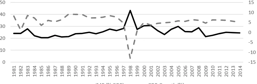
income. As evidenced by Wijayanti (2005) and Revania (2014), GDP has positive impact and significantly affects to import. Figure 1 shows that the proportion of imports to GDP during 1981-2014 tended to be stable. However, there is a distortion when shocks occur in domestic economy. On the other hand, shocks in domestic economy lead to lower GDP growth (below 5%). Meanwhile, import activity becomes a solution to recover from domestic economic shocks. Moreover, import policy is made to curb inflation. Pramaboyu (2007) showed that inflation has positive impact and significantly affects to import value. Inflation can occur as a result of increasing demand (demand pull inflation) and imbalance of resource capability to meet the demand. If the result presents Qd > Qs, the economic actors need to increase the supply of goods through imports. The inflation may cause some bad effects for the economy. Sukirno (2012) stated that inflation might worsen the long-term growth prospects, reducing real incomes of workers with fixed salaries and reducing the value of wealth in the money form, and might worsen the income distribution.
As overlooked from the population, Indonesia is generally reckoned as a great
country. Indonesia’s average population growth
during 1981-2014 was about 1.604% (World Bank, 2016) and showed a negative trend. Import activities are essentially required once the
-15
Source: World Development Indicators, World Bank (2016)
domestic produres are unable to meet the demand. Adewuyi (2016) mentioned that the population contributed a significant impact on import demand in the long term.
In addition, a country will import goods when it has a large amount of total reserves. The huge total reserves can convince the importers to make a purchase with debt mechanism. Furthermore, Mankiw (2010) stated that total reserves contributed as one of the factors that influence the exchange rate which later affects the international trade, as evidenced by Pramaboyu (2007).
Based on the previous explanation, it is believed that imports remain important for Indonesia. Imports could occur to stimulate economy (Wijayanti, 2005); (Revania, 2014), to curb inflation (Pramaboyu, 2007), and to recover from domestic economy shock. Moreover, import capacity is believed to be influenced by the growing population (Adewuyi, 2016) and the growing total reserves. However, there have been limited studies concerned on the factors affecting Indonesia imports both for short and long term. Therefore, this research intends to analyze the factors affecting Indonesia imports both in short and long term.
RESEARCH METHODS
Research on the analysis of Indonesia imports is directed to study the factors that influence variation in Indonesia imports. This research applies time series data for 34 years (1981-2014). This type of data is secondary data obtained from the World Development Indicators published by the World Bank.
The approach used in the research is the Error Correction Model / ECM which is selected since the data is stationary at first difference level and shows the balance in the long term/cointegrated. Widarjono (2016)
stated that if the error coefficient of imbalance is statistically significant then the ECM model specifications is valid. ECM model used in this research is Engle-Granger model which can be formulated in the following equation.
D (IMPt) = 1 + 2 D (GDPGROWTHt) +3 D (DSHOCKt) + 4 D(INFt) +5 D(LPOPt) + 6
D(TRSVt) +β7 ECt + et………(1)
Equation (1) is a short-term model. From equation (1), an estimated long-term regression coefficient can be formulated as in the following equation (2).
IMPt = 1 + 2 (GDPGROWTHt) +3 DSHOCKt + 4 INFt +5 LPOPt + 6 TRSVt + et…….…(2)
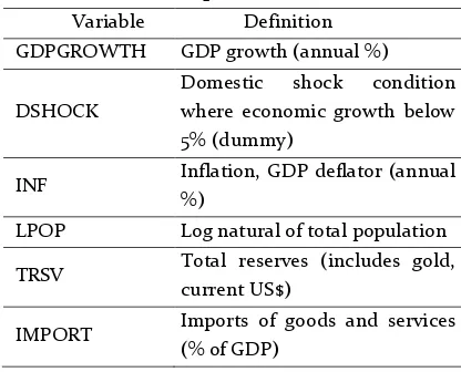
Meanwhile, the operational definition for each variable can be seen in Table 1.
Table 1. Operational Definition Variable Definition
GDPGROWTH GDP growth (annual %)
DSHOCK
Domestic shock condition where economic growth below 5% (dummy)
INF Inflation, GDP deflator (annual %)
LPOP Log natural of total population
TRSV Total reserves (includes gold, current US$)
IMPORT Imports of goods and services (% of GDP)
Source: Researcher, 2016
RESULTS AND DISCUSSION
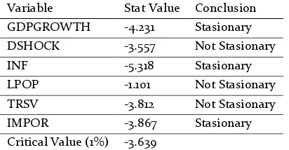
to change (Effendi and Setiawan, 2014). Stationary test data in this study is conducted by applying the unit root test model method of Augmented Dicky-Fuller (ADF). In order to determine whether the condition is a stationary, the author conducts a comparisson between the value of the ADF statistic and the critical value of the statistical distribution of Mackinnon. If the absolute value of the ADF statistic is greater than the critical value then the data observed shows stationary. Using Eviews9, stationary test results are shown in the following Table 2.
Table 2. Unit Root Test Results at the Level Variable Stat Value Conclusion GDPGROWTH -4.231 Stasionary DSHOCK -3.557 Not Stasionary
INF -5.318 Stasionary
LPOP -1.101 Not Stasionary
TRSV -3.812 Not Stasionary
IMPOR -3.867 Stasionary
Critical Value (1%) -3.639
Source: Operation Results in Eviews9, 2016
Based on the stationary test results in Table 2, the variable of economic growth, inflation and the import are stationary at the current level whereas the dummy variable shock, log population and total reserves are
not stationary at α = 1%. Therefore, the degree
of integration testing is required to determine if the previous data is not stationary at the first difference. This test is shown in Table 3.
Table 3. Unit Root Test Results at the First Difference Level
Variable Stat Value Conclusion
DSHOCK -8.390 stationary
LPOP -5.884 stationary
TRSV -4.453 stationary
Critical Value (1%) -3.639
Source: Operation Results in Eviews9, 2016
After testing the degree of integration with the critical value of 1%, the result is the value of the dummy variable ADF shock, log population, and total reserves are smaller than the critical value. It can be concluded that all variables are stationary at first difference level. In the end, all variables have been stationary which can be applied as input to the model.
In this research, cointegration test is conducted by using Cointegration Regression Durbin-Watson (CRDW). The first stage is conducted to estimate the regression model and to obtain the DW value. Later, the DW value is
compared with α = 1%, α = 5%, α = 10%, in which
the amount of each is 0.511; 0.386; and 0.322. If the calculated d-value is greater than the critical value, then the data is cointegrated (Widarjono, 2016). Table 4 is the result of CRDW.
Table 4. Cointegration Regression Durbin Watson (CRDW) Result
Regression Equation Calculated CRDW
Critical Value α=5% IMPOR=GDPGROWTH,
DSHOCK, INF, LPOP, TRSV
1.2149 0.386
Source: Operation Results in Eviews9, 2016
Table 4 shows that CRDW value is greater
than the absolute critical value at α = 5% (1.2149>
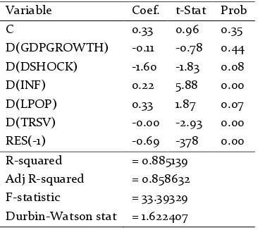
Table 5. ECM Estimation Results Variable Coef. t-Stat Prob
C 0.33 0.96 0.35
D(GDPGROWTH) -0.11 -0.78 0.44 D(DSHOCK) -1.60 -1.83 0.08
D(INF) 0.22 5.88 0.00
D(LPOP) 0.33 1.87 0.07
D(TRSV) -0.00 -2.93 0.00 RES(-1) -0.69 -378 0.00 R-squared
Adj R-squared F-statistic
Durbin-Watson stat
= 0.885139 = 0.858632 = 33.39329 = 1.622407 Source: Processed Data
Based on the results in Table 5, the formula is written in the following equation.
D(IMP) = 0.33 - 0.11 D(DGDPGROWTH) -1.60 D(DSHOCK) + 0.22 D(INF) + 0.33 D(LPOP) - 1.33E-10 D(TRSV) - 0.69 RES(-1) ...…………(3)
It is revealed that the independent variables can explain the dependent variable. RES (-1) coefficient is called as the speed of adjustment which result is negative and significant. This indicates that the error correction model is valid and can be used to analyze the factors that affect the import of Indonesia. In addition, it is revealed that the
inflation variable and trsv are significant at α
= 5%. Meanwhile, dshock and lpop variables
are significant at α = 10%. Furthermore, the
long-term estimates can be formulated in the following equation.
IMP = 18.9268 – 0.0827 GDPGROWTH – 0.0844 DSHOCK + 0.2248 INF + 0.4072 LPOP
– 3.92E-11 TRSV ………...………(4) Adj R2=0.767, F-stat=22.69, DW=1.215
The variable of inflation, lpop, and trsv
are significant at α = 5%.
Classic Assumption Test, consist of liniearity, multicoliniearity, normality, heteroscedasticity, autocorelation. One of the assumptions or the proposed restriction is linear on its parameters. However, in many economic cases, there are possibilities that are not linier in the parameters or are even possible on a variable (Ekananda, 2015). The linearity test is used to see whether the model has a linear relationship. Null hypothesis/H0 suspects that the model is linear in its parameters. Linearity test in this research applies the method of Ramsey Reset Test. A model can accept H0 if the probability of F-statistic value is more than the selected critical value. Based on the results of Ramsey Reset Test, it is demonstrated that the value of Prob F on the short-term model (0.7229), and long term (0.3815) is greater than the selected critical value (0.01). Therefore, the null hypothesis is accepted which can be concluded that the model is linear in its parameters.
Multicolinearity test is used to determine the existence of a perfect linear relationship among the explanatory variables. Multicolinierity might cause errors in variants on the model; therefore, the value of t-statistic is very small and insignificant. On the other hand, the sign in the regression model is often contrary to its underlying theory (Ekananda, 2015). Multicolinierity detection used in this research is the Variance Inflation Factors (VIF). Multicolinierity occurs if the value of Centered VIF is more than 10. Based on the VIF Test, the value of all independent variables in the model, both short-term and long-term, is less than 10. In sum, it can be concluded that the models are free from multicolinierity.
residuals and is normally distributed. Ekananda (2015) stated that small probability value leads to the rejection of the null hypothesis of normal distribution. Based on the JB normality test, it appears that probability value in both short-term and long-term models has exceeded the error rate (1%). Thus, null hypothesis is accepted, and the data are normally distributed.
Classical assumption assumes that the variance of the element of disturbances/error is a constant number or homoscedastic. This assumption is a consequence of being unable to meet the other classical assumptions which are the zero conditional mean or zero error expectation (Wahyudi, 2016). However, the variance of the error is not always constant for each observation. The estimation results become inefficient since the variance is over the estimation. This implication makes t statistics and F statistics to be very small and insignificant. Therefore, t test and F test can be useless/misleading (Ekananda, 2015). Detection of heteroscedasticity used in this research is the Glejser method. Null hypothesis assumes that the error variance is constant (homoscedastic) and is acceptable if the prob. value is more than the selected significance level. Based on Glejser method, in both short-term and long-term model, all
variables are not significant at α = 1%.
Therefore, the null hypothesis is accepted and the author concluded that the model is homoscedastic.
One of the classic assumptions related to the disturbance variable is the absence of relationships among error variables. Literally, autocorrelation means the correlation between the member's observations and other different observation time (Widarjono, 2016). However, Sumodiningrat (2013) states that the autocorrelation might also occur in a series of observations that is arranged in
spacial series. Serial correlation will produce an inefficient estimation because the produced variance is not the actual value (variance under estimate). According to Ekananda (2015), autocorrelation will make the estimation result error to be smaller than the actual standard error which leads to the rejection of the null hypothesis. Autocorrelation test method used in this research is Breusch-Godfrey Serial Correlation LM where the null hypothesis is no autocorrelation. Autocorrelation test results on the short-term model and the long-term model indicate that Prob. Chi-Square (2) is not significant at 1% significance level. Then the null hypothesis is accepted, and it can be said that the model is free of autocorrelation.
The t-test is used to determine the effect of each independent variable on the dependent variable. This study used a two-sided t test. If the statistic is t> t table then the independent variables affect the dependent variable, and vice versa. Table 5 is the result of the t-statistic model of short-term and long-term.
Table 5. Result of t-statistic Test
Variable Result
C Has No Effect
D(GDPGROWTH) Has No Effect D(DSHOCK) Has influence**
GDPGROWTH Has No Effect
domestic economic shocks, inflation, population, and foreign exchange reserves. In the long run, variables affecting demand for imports are inflation, population, and foreign exchange reserves. In addition, the variable RES (-1) significantly affects the Indonesia imports. This indicates that the speed of adjustment is valid and can be used to adjust the imbalance errors in the short term.
F test is used to determine the simultaneously influence of independent variable on the dependent variable. Based on the estimation, it is indicated that the short-term F-statistic is 33.39329, and the long short-term F-statistic is 22.68686, exceeding the value of F table with a significant level of 5% by 2.56. Therefore, H0 is rejected and Ha is accepted. In sum, the economic growth variables, dummy shock, inflation, population logs, and foreign exchange reserves simultaneously affect the import of Indonesia from 1981 to 2014.
According to the regression results, it is revealed that the short term Adjusted R-square value is 0.858632. This value indicates that economic growth, dummy shock, inflation, population logs, and total reserves could explain the variation of demand imports of goods and services in Indonesia by 86% while the rest of 24% is explained by other variables outside the model. Adjusted R-square value in the long term is 0.766676. This value indicates that economic growth, dummy shock, inflation, population logs, and total reserves could explain the variation change of imports of goods and services in Indonesia by 77%. Meanwhile, the rest of 23% is explained by other variables outside the model.
Based on the speed of adjustment, there is a 69% imbalance in the short-term affecting the independent and the dependent variable
corrected in every period. Both in short-term and long-term model, the variable of GDPGROWTH and Indonesia economic growth seen from GDP growth have no significant effect on the proportion of imports to GDP for Indonesia. It is revealed from the absolute value of the t GDPGROWTH variable on short-term and long-term model, each of which has a value of 0.774379 and 0.368015 being smaller than t table
(α = 5%) of 1.701. This finding is contrast to the
results of research as conducted by Wijayanti (2005) and Revania (2014).
In the short term, at a significant level of α
= 10%, DSHOCK variables (Dummy Shock) significantly affect the Indonesia imports. DSHOCK variable coefficient is -1.60615 meaning that the proportion of imports to Indonesia's GDP on average will be lower at 1.60615% of the total GDP when domestic economic shocks occur (ceteris paribus). Yet, DSHOCK variable coefficient in the long term equals to -0.84395 with absolute t-statistic of 0.677358 <t-table (α = 5%) was 1.701. Under the terms of statistics, it can be seen that the shock Dummy variables did not significantly affect the proportion of imports to Indonesia's GDP in the long term. This indicates that the economic turmoil in the country provides significantly negative effect on the proportion of Indonesia imports to GDP in the short term, whereas in the long term, it has no significant effect. Domestic shocks require economic actors to adjust and restore the economy quickly. One of the actions that can be undertaken is to reduce imports. However, in a series of data, imported components would have a major proportion of GDP when the domestic economic shocks occur. Thus, the import policy is carried out as economic stimulus.
Indonesia imports can be evidenced by the t-statistic value of 5.880426 which is greater than t-table value of α = 5% at 1.701. This result indicates that inflation has a positive and significant impact on the proportion of imports to Indonesia's GDP. If other variables are assumed to be constant, the proportion of imports to Indonesia's GDP on average will increase by 0.223684% to the total GDP while inflation rose by 1%. In the long run, inflation has a coefficient of 0.224832 with a t-statistic of 3.694089. In statistical conditions, the effect of inflation to the proportion of imports to Indonesia's GDP can be evidenced by the value of t-statistic (3.694089> t-table), and
the value of α = 5% is 1.701. This result suggests
that in the long run, inflation provides positive and significant impact to the proportion of imports to Indonesia's GDP. Inflation affects imports because import policy becomes a solution to curb inflation. The greater the inflation, the greater the import would be. The result in this study is in line with the research that had been conducted by Pramaboyu (2007).
The estimation results indicate that in the short term, LPOP variable (population growth) has a coefficient of 0.326543 with a t-statistic of 1.872063. In t-statistical conditions, the effect of population growth on the proportion of Indonesia imports can be evidenced by the value of t-statistic 1.872063 > t-table 1.701. These results indicate that population growth has a positive and significant impact to the proportion of imports to Indonesia's GDP. If other variables are assumed to be constant, the proportion of imports to Indonesia's GDP on average will increase by 0.326543% of the total GDP if the population growth has increased by 1%. In the long term, the value of the coefficient is 0.407203 and the value of t statistic 3.864180 higher than t-table 1.701. This result indicates
that, in the long term, population growth has a positive and significant impact to the proportion of Indonesia imports. The author assumes that this estimation also indicates that the increasing population in Indonesia is not accompanied by the increasing dominance of technology, as in line with the assumption of the Malthusian theory. In the case of Indonesia, when the population increases, it is necessary to import due to the demand excess. The findings in this research support the research that has been conducted by Adewuyi (2016) with the research object in Nigeria.
TRSV Variable (foreign reserves) in the short term has a coefficient of -1.33E-10. At the
significant level α = 5%, international reserves
significantly influence the proportion of Indonesia imports. The statement can be viewed through the absolute value of the t-statistic (2.927950) which is greater than t-table (1.701). If other variables are assumed to be constant, the increase in foreign reserves which equals to 1 US $ on average will reduce the proportion of imports amounted to 0.000000000133% of Indonesia's GDP. In the long term, the coefficient of reserves is -3.92E-11 with the absolute t-statistic amounted to 2.318151 > t-table
(α = 5%) of 1.701. It is suggested that in the long
term, the increasing foreign exchange reserves have negative and significant impact to the proportion of Indonesia imports. Contrastingly, the increasing foreign exchange reserves in Indonesia are not intended to increase imports. The additional reserves are applied to strengthen the domestic economy reducing the imports.
CONCLUSIONS
In the short term, there is a difference in the proportion of imports when economic shocks occur. However, in the long term, there is no difference between the presence and absence of shocks to the proportion of Indonesia imports. Inflation is proven to have a positive and significant impact to the Indonesia imports both in the short term and long term.
Population growth is proven to have a positive and significant impact to the Indonesia imports both in the short and long term. The foreign exchange reserves also show to have a negative and significant impact to the Indonesia imports both in the short and long term.
For further research, other researchers can discuss more deeply about the linkage of economic growth with imports. In addition, further categorization of imports can be divided into two: before the crisis and post crisis.
REFERENCES
Adewuyi, A. O. (2016) ‘Determinants of import demand for non-renewable energy ( petroleum ) products : Empirical evidence from Nigeria’,
Energy Policy. Elsevier, 95, pp. 73–93. doi: 10.1016/j.enpol.2016.04.035.
Carbaugh, R. (2005) International Economics. 10th edn. Washington: Routledge.
Dunn, R. M. and Mutti, J. H. (2004) International
Economics. 6th edn. New York: Routledge.
Effendi, N. and Setiawan, M. (2014) Ekonometrika:
Pendekatan Teori dan Terapan. Jakarta: Salemba
Empat.
Ekananda, M. (2015) Ekonometrika Dasar Untuk Penelitan Ekonomi, Sosial, dan Bisnis. Jakarta: Mitra Wacana Media.
Jechlitschka, K., Kirschke, D. and Schwarz, G. (2007)
Microeconomics Using Excel: Integrating Economic Theory, Policy Analysis and Spreadsheet Modelling. New York: Routledge.
Mankiw, G. (2010) Macroeconomics. 7th edn. New York: Worth Publisher.
Pramaboyu, I. (2007) ‘Pengaruh Nilai Tukar, Inflasi, dan Nilai Ekspor Terhadap Nilai Impor’. Malang: FEB UB.
Revania, L. (2014) ‘Analisis faktor-faktor yang
mempengaruhi impor jagung di indonesia tahun 1982 –2012’, Journal of Economics and Policy, 7(1), pp. 102–112. doi: 10.15294/jejak.v7i1.3847.
Rosyidi, S. (2001) Pengantar Teori Ekonomi: Pendekatan kepada Teori Ekonomi Mikro & Makro. Jakarta: RajaGrafindo Persada.
Sukirno, S. (2012) Makroekonomi Teori Pengantar. 3rd edn. Jakarta: Rajawali Press.
Sumodiningrat, G. (2013) Ekonomi Pengantar. 2nd edn. Yogyakarta: BPFE.
Wahyudi, S. T. (2016) Konsep dan Penerapan Ekonomotrika
Menggunakan E-Views. Jakarta: Rajawali Press.
Widarjono, A. (2016) Ekonometrika: Pengantar dan
Aplikasinya disertai Panduan Eviews. 4th edn.
Yogyakarta: UPP STIM YKPN.
Wijayanti, N. (2005) The Stability Analysis of Import Function on 1985-2003: Case Study in Indonesia.
Unpublished Minor Thesis. Under-Gradute
Programme. Malang: FEB UB.
World Bank. (2016) World Development Indicators.http://data.worldbank.org.