A Robust Motion Detec tion Technique for Dynamic Environment Monitoring

Digital Object Identifier 10.1109/MRA.2013.2297812 Date of publication: 10 March 2014

A Robust Motion

Detec tion Technique for

Dynamic Environment

Monitoring

A Robust Motion

Detec tion Technique for

Dynamic Environment

Monitoring

By Qadeer Baig, Mathias Perrollaz, and Christian Laugier

A Framework for Grid-Based

Monitoring of the Dynamic

Environment

T

he Bayesian occupancy filter (BOF) provides a framework for grid-based monitoring of the dynamic environment. It allows us to estimate dynamic grids, containing both information of occupancy and velocity. Clustering such grids then provides detection of the objects in the observed scene.

In this article, we present recent improvements in this framework. First, multiple layers from a laser scanner are fused using opinion pool, to deal with conflicting information. Then, a fast motion detection (MD) technique based on laser data and an odometer/inertial measurement unit (IMU) infor-mation is used to separate the dynamic environment from the static one. This technique is based on transferring occupancy informa-tion between consecutive data grids, instead of performing a complete simultaneous localization and map-ping (SLAM) solution. The objective of the MD technique is to avoid false posi-tives (static objects) like other detection and tracking of moving objects (DAT-MOs) approaches. Finally, we show the integration with BOF and with the subse-quent tracking module called the fast clus-tering tracking algorithm (FCTA). We show the improvements achieved in tracking results after this integration, for an intelli-gent vehicle application.

Moving Objects Detection for Risk Assessment

In the field of advanced driver assistance sys-tems (ADAS), many current approaches rely on the perception of the road scene. Particularly,

the detection and tracking of the objects in the scene are essen-tial for prediction of risky driving situations. Among recent approaches for risk estimation, the authors of [1] proposed to model and recognize the behavior of road scene participants to refine the prediction of their future trajectories. It allows a long-term prediction, compared with classical geometric approaches. This is promising for long-term risk assessment, but reasoning on behaviors requires us to separate the environment into static and dynamic parts.

A huge amount of work has been done to detect moving objects, especially by the vision community [2]–[5]. These techniques have primarily been based on background sub-traction or motion cues. Similar techniques have also been used in occupancy grids to detect moving objects [6], [7]. These techniques are based on inconsistencies observed for new data by comparing them with maps constructed by SLAM. The authors of [8] and [9] have also proposed model-based techniques to detect moving objects on the roads in the context of autonomous vehicle driving. More recently, Demp-ster–Shafer theory-based grids (evidential grids) have been used to detect moving objects using conflict analysis tech-niques [10], [11]. However, finding appropriate values of the operators involved is usually a challenging task. The tech-nique described in [12] uses a modified concept of particle fil-ers to monitor dynamic environment.

Various approaches exist for classifying the environment. Computing a precise map of the environment, coupled with an accurate localization algorithm, can be computationally costly. Thus, performing a SLAM-based localization would be more realistic for commercial vehicles, since the computed occupancy grid [13] provides a description of the static envi-ronment. More elaborate techniques like [7] or [8] improve this approach by performing detection and classification simultaneously in a model-based tracking framework.

When considering the problem of DATMO, many differ-ent methods have been proposed in the literature. Petrovs-kaya et al. [14] propose to classify these methods in three cat-egories: 1) traditional DATMO, 2) model-based DATMO, and 3) grid-based DATMO. For the purpose of this article, we are only interested in using grid-based DATMO.This method is based on the use of the BOF originally developed in [22] and then expanded in [15] and [16], combined with a FCTA [17] for monitoring the dynamic environment. An important work to cite here is [18]. The idea was inspired by the original BOF formulation [22], but it also integrates prior map knowl-edge. This new formulation has comparable results to that of the original BOF framework, but it lacks the static/dynamic division of the cells.

Although the BOF and FCTA combination works fine for properly tuned FCTA parameters, finding appropriate values for these parameters can be time consuming. Without proper parameter values, FCTA may miss true tracks (for bigger parameter values) or may give false tracks (for smaller param-eter values). The set of paramparam-eters of FTCA cannot be pre-cisely tuned for moving objects detection, since at the output of the BOF it must deal with both static and dynamic

envi-ronments.The BOF framework performs the environmental monitoring even when no motion sensor is available. Since the objective of the FCTA is to cluster and track the moving objects, it is advantageous to remove the static parts from the output of the BOF and input the FCTA only with detected moving parts. If input of the FCTA only consists of likely moving parts of the environment, the dependence of FCTAs performance on the values of its parameters can be relaxed.

In this article, we first present our new approach for building occupancy grids from multiple layers of laser scans. Then, we propose a fast and efficient method for static/dynamic environment classification from the occupancy grid generated in the last time-step and show its integra-tion within the BOF framework, to provide a more accurate representa-tion of cell velocities. The BOF also takes the occu-pancy grid generated by

the fusion module as an input, and outputs an occupancy and velocity grid that is used by the FCTA. Therefore, we also pres-ent the integration of our approach with the FCTA. This inte-gration has enabled us to remove a large number of false tracks. Our approach is different from other grid-based meth-ods in the sense that a complete SLAM solution is usually implemented to separate the moving parts from the static parts (as in [9]).In this article, we have developed a technique that uses only a few consecutive frames to detect moving parts rapidly, and can be easily implemented in real time.

The BOF Framework

In this section, we briefly introduce the BOF framework with the FCTA module to detect and track the moving objects. In this framework, the idea is to perform sensor fusion and envi-ronment monitoring at a low level, hence the fast and efficient grid-based representation used during all the processes. Data association is delayed to avoid association-related problems during the early stages. The objects are only retrieved at the end of the processing through clustering of the dynamic grid. To summarize, the complete processing from sensor data to objects can be divided into three stages: 1) multisensor fusion using occupancy grid representation, 2) filtering and estima-tion of dynamic grid, and finally 3) clustering of the dynamic grid and tracking.

Sensor Fusion From Multiple Lidar Layers

Multiple layers of laser scans could be provided either by a multiple-layers laser scanner or by multiple single-layer laser scanners. Each layer can be used to compute an occupancy grid using the classic range finder probabilistic sensor model

We have developed a

technique that deals with

only a few consecutive

frames to detect moving

parts rapidly, and can

easily be implemented

described in [19]. To retrieve a single grid to represent the environment, the data from all these layers are merged using the approach described in [20].This approach fuses the sen-sory information by using linear opinion pools [21].

The principle is to generate a posterior distribution over the occupancy of a cell C of the grid given the opinion of m sen-sors "Y1fYm,. For each cell, a sensor gives two quantities: 1) its estimation for the occupancy of the cell P^C;Yih and

( ),

w Ci and 2) a measure of the confidence for such

estima-tions. The idea is to shutdown those sensors that do not give relevant information to the process by assigning a low weight to them. The fusion of all sensory information will be as follows:

( ) ( ),

P C Y1 Y w C P C Y

1

m i i

i m f

; ₌a ;

=

^ h

/

(1)

where _{i 1}w Ci( ) 1

m

a₌

=

-8

/

B is a normalization factor for the weights. Equation (1) is used to generate two-dimensional occupancy grids. For each sensor Yi we must define

,

P C Y^ ; ih the probability of a cell being occupied given the

sensor information, and w Ci( ), the confidence on the opin-ion. The confidence includes two components: one related to the geometry (e.g., if the beam is close to the ground), and

one related to the probability of the cell to be actually visible by the sensor (details in [20]). Note that we assume indepen-dence among cells, to be efficient in computing (1), for each cell in parallel.

There are two advantages with this method. First, the con-fidence on occupancy is computed independently for each cell of the grid. Therefore, if a layer hits the road surface, the confidence will be low and it will not interfere with other lay-ers. Second, it has the advantage of reducing the errors due to conflicting information from the multiple layers. An example of such conflictual information appears when a layer hits an object (meaning that the corresponding cell is occupied) while an upper layer goes over the object (meaning that the cell is free). As seen in Figure  1, standard Bayesian fusion would lead to low occupancy probability, while the proposed approach would see the cell as probably occupied.

Filtering the Grid Using the BOF

The BOF provides filtering capability, as well as the ability to estimate a velocity distribution for each cell of a grid. It is an adaptation of the Bayesian filtering methodology to the occu-pancy grid framework, based on a prediction-estimation para-digm, as shown in Figure 2. As an input, it uses an observed occupancy grid. On its output, it provides an estimated occu-pancy grid as well as a set of velocity grids, representing the probability distribution over possible velocities for each cell.

In this article, the prediction step propagates cell occu-pancy and velocity distributions of each cell in the grid and obtains the prediction (P O Act ct), where ( )P Oct denotes the

occupancy distribution and ( )P Act denotes the antecedent

(velocity) distribution of a cell c at time .t The velocity of a cell depends on its previous position called antecedent, if we know the previous position of a cell, we can calculate its velocity because the size of the cells is fixed and we know the time interval as well. In the estimation step, (P O Act ct) is updated by considering the observations yielded by the sen-sors

%

_iS₌₁P Z^ it;A Oct tch to obtain the posterior state estimate

,

P O A^ ct ct;6Z1tgZtS@h where Zit denotes the observation of

sensor i at t. This allows us to compute by marginalization P O^ ct;6Z1tgZSt@h and P A^ ct;6Z1tgZSt@h, which will be used

for prediction in the next iteration. (a)

(c) (b)

Figure 1. (a) The left-hand-side image from the stereo camera. (b) Occupancy grids computed from multiple layers of laser scans with Bayesian fusion. (c) Occupancy grids computed from multiple laser scans with our new approach. Due to conflicting information, the left fence disappears with Bayesian fusion, while still being visible with our method. (Photos courtesy of INRIA.)

Estimation z Prediction

P(Ot c A

t c)

P(Zt ;Ot_c At_c)

P(Ot

c Atc;[Zt =z])

Detecting Objects with the FCTA

While the dynamic grid representation provided by the BOF can be sufficient for some applications (e.g., navigation), moving object detection must retrieve an object level repre-sentation of the scene.This cannot be directly reached from the occupancy grid, and therefore a clustering algorithm is necessary. An algorithm adapted to the BOF framework is the FCTA described in [17]. This algorithm is able to create clusters based on the connectivity in the occupancy grid, as well as the Mahalanobis distance between cells in the esti-mated velocity grids.Thus, two connected cells with different velocities are not merged during the clustering process. This is very important because two closely located clusters may actually belong to two different objects moving with different velocities. Thus, the FCTA elegantly addresses the partial occlusion problem.

FCTA includes a Kalman filter for target tracking and a region of interest (ROI) prediction approach that allows com-putation to be performed in real time. The output of the algo-rithm is a set of tracked objects with position, velocity, and associated uncertainties.

The integration of this detection and tracking algorithm with the BOF algorithm provides a single application that takes its input from the installed sensors and outputs the tracks to be used for risk assessment. Like other approaches, FCTA also suffers from a false tracks detection problem, so a preclassification of cells into static and dynamic categories can help in this article. The MD module capable of classifying the environment into static and dynamic regions can also help fix the false tracks detection problem.

Motion Detection

Outline of the Approach

In this section, we detail the technique that we have devel-oped to find moving parts of the environment. This MD module is situated in the processing chain just before the BOF. The input to this module consists of an occupancy grid generated by the fusion module, described in the previous section. Let us represent this occupancy grid at time t as OGt

and an ith cell in this grid can be accessed as OG it[ ] where

i N

0# 1 _{with N being the total number of cells of this} occupancy grid. The value of each cell of this grid is between 0 and 1, i.e., 0#OG it[ ]#1, and represents the internal belief of the ego vehicle about the occupancy state of each cell. Zero means empty and 1 means occupied.

The module also requires proprioceptive information from the vehicle. Here, we consider using an IMU, which pro-vides at time t—along with other information—two compo-nents of velocity vt=( , )v vx y and the values of quaternion

components for orientation Qt=( , , , ) .q q q q0 1 2 3 From this information, we calculate the translational and rotational velocities ut=( ,vtwt) of the vehicle

.

v v2 v2

t= x+ y (2)

To compute rotational velocity of the vehicle, we calculate yaw angle of the vehicle from the quaternion as

( ( ),

( )) .

tan

y a q q q q

q q q q

2 2 0 3 1 2

1 2 2 2 3 3

) ) )

# ) ) )

= +

- + (3)

If dt is the time difference between two successive data frames at time t and t-1, then rotational speed w at time t is equal to the yaw rate given as

. w

dt

y y 1

t

t t

= - - (4)

MD Algorithm

At each time ,t the algorithm consists of following steps.

Step 1: Free and Occupied Count Arrays

For each new input occupancy grid OGt we create two count

arrays having the same dimensions as that of OGt, the first one called FreeCountt and the other called OccupiedCount ,t to

keep count of the number of times a cell has been observed “free” and number of times it has been observed “occupied,” respectively. These arrays are initialized from OGt as

OccupiedCount [ ] , if [ ] .

, otherwise

i 1 OG i 0 5

0

> t

t

=) (5)

and

OG_t

OG_t -1

O_t-1 O_t

P

FreeCount [ ] , if [ ] .

Step 2: Counts Update from Previous Step

Suppose FreeCountt-1 and OccupiedCountt-1 are the updated count arrays at time t-1. We want to update new counts FreeCountt and OccupiedCount .t Since the vehicle

has undergone a position change determined by ut=( ,v wt t), there is no direct correspondence between cells of the occu-pancy grids OGt and OGt-1. We must find the transforma-tion that maps a cell in OGt-1 to a cell in OGt using .ut This

situation is shown in Figure 3, where OGt-1 has origin at Ot-1 and OGt has origin at Ot. To find the transformation

suppose Ot-1=(xt-1,yt-1,it-1)=( , , )0 0 0 is the pose (posi-tion and orienta(posi-tion) of the occupancy grid at time t-1 (i.e., of OGt-1) and we want to find Ot=( , , ),x yt t it the pose of

OGt under .ut Consider a circular motion trajectory, meaning

that the object with both linear and rotational velocity is sup-posed to move along the circular path. For short periods of time, it can be an acceptable approximation. Then, the pose of Ot with respect to Ot-1 is given as

Although it is a good approximation for a relatively accurate motion sensor, localization errors may occur due to sensor uncertainty and external factors (like vehicle slipping). To fix these problems, we use a pose correction measure similar to the one given in [19]. In this correction measure, ROI is defined around the new position at time t [given by (7)] and calculated using the circular motion model. Different pose samples are taken from this region and for each pose sample, a scorefunc-tion is evaluated using new data OGt and free and occupied

counter values. The function is given as (OC for occupied counter, FC for free counter, and N for total grid cells)

score

, if ( [ ] . ) and

(OccupiedCount [ ] FreeCount [ ]) , if ( [ ] . ) and

(OccupiedCount [ ] FreeCount [ ]) , otherwise. cell is occupied or empty.) Here i and j are corresponding cells in occupancy grids at t-1 and ,t respectively, as explained below. The pose sample giving the highest value of this score is taken as the correct current pose of the vehicle improving the overall MD results.

An important thing to note here is that we are concerned with the localization of only a few consecutive frames. We do not solve the complete SLAM problem, making the technique very fast. The pose estimation between two frames may not be exact, but the error does not accumulate over longer

peri-ods of time because the map is very local, restricted to one small window of one data frame. The ego vehicle is always located on the middle point of the bottom edge.

To map a cell of grid OGt-1 to grid OGt, we proceed as

fol-lows. Suppose point P (shown in Figure 3) is the center of a cell in grid OGt-1 and we want to find its corresponding cell in grid

.

OGt We define the following two pose manipulation operations.

Combination values, we can easily calculate the index of the cell where point P lies in grid OGt. These transformations will map a cell having index i in OGt-1 to a cell having index j in grid

.

OGt If this cell j is visible in OGt, i.e., 0#j<N, then we

can update new count values for this cell as

FreeCount [ ]t j =FreeCount [ ]t j +FreeCountt-1[ ],i (13) and (OCount in the following equations is OccupiedCount to fit the equation in a line)

OCount [ ]t j =OCount [ ]t j +OCountt-1[ ] .i (14) We repeat this process for all cells of grid OGt-1 to update count values in grid OGt.

Step 3: Motion Detection

MotionGrid [ ]

Here m is a sensor specific input parameter, and its empirically learnt value in our experiments is 2. Therefore, a cell has a moving object in it if it is occupied at current time instant and previously it was observed as free for a suffi-cient number of times (at least twice the number of times it has been observed as occupied). After this processing, MotionGridt has 1 in the cells, which are detected as

belonging to moving objects.

The final measure that we have taken to remove false pos-itives is the implementation of a road border detection tech-nique (as detailed in [23]). In this techtech-nique, road borders are searched along directions that are parallel to the current vehicle orientation, using a window-based approach. The windows containing more occupied cells than the specified threshold signals the presence of a road border. When road borders are detected with high confidence, moving cells detected beyond the road border are ignored.

Integration with the BOF Framework

We have updated the BOF implementation to consider the MD results. The motion grid is used as an input for updating the BOF. If the input motion grid indicates that a cell belongs to a static object, then the cell’s velocity distribution over the velocity range is set to uniform for all discrete velocity values during the prediction and update cycles of BOF. This essen-tially means that no velocity information for a given cell is available and the cell is labeled as static in the current BOF

implementation. However, if the cell has been detected as belonging to a moving object, then the velocity distribution prediction and the update cycle are carried out normally. In formal terms as outlined in [17], this change in the paramet-ric form of dynamic model can be stated as:

( | )

parameter of BOF, modeling the prediction error probability. The antecedent of a cell i at time t means the cell j at time t-1 where the same object (currently seen in cell i) was seen. This knowledge along with the knowledge of time dif-ference and cell sizes lets us calculate the object velocity. A complete derivation of this equation can be found in [17].

IMU Data

Figure 4. A block diagram of the MD system.

(a)

(b) (c)

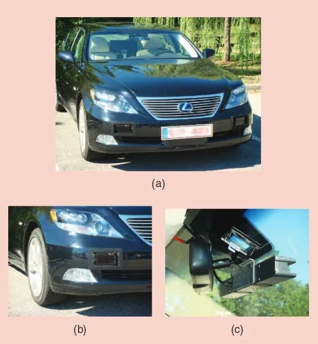
Figure 5. (a) The Lexus LS600h, equipped with (b) two IBEO Lux lidars and (c) a TYZX stereo camera. (Photos courtesy of INRIA.)

(a) (b)

Integration with FCTA

We have also updated the FCTA implementation to consider the MD results. The cells, which do not possess the velocity information, are now ignored during the clustering step. While most of the areas belong to static objects and are detected as static by the MD module, two main advantages are expected from this strategy: 1) the clustering stage of the algorithm is highly accelerated by the reduction of hypotheses and 2) the wrong moving clusters are ignored because they are not con-sidered for clustering, even with the relaxed FCTA parameters. A block diagram of the system is shown in Figure 4.

Experimentation

Experimental Platform

Our experimental platform is a Lexus LS600h car, shown in Figure 5. The car is equipped with the following sensors (shown in Figures 5 and 6): two IBEO Lux lidars placed in the

front bumper, a TYZX stereo camera situated behind the windshield, and an Xsens MTi-G sensor (IMU with global positioning system). Extrinsic calibration of the sensors is done manually for this article. Using the grid-based approach and considering the resolution of the grid, a slight calibration error has little impact on the final results.

The hardware specifications include an IBEO Lux Lidar laser scanner that provides four layers of up to 200 beams with a sampling period of 40 ms. The angular range of each lidar is 100c, and the angular resolution is . .0 5c The on-board computer is equipped with 8 GB of random access memory, an Intel Xeon 3.4-GHz processor, and a NVIDIA GeForce GTX 480 for GPU. The observed region is 60 m # _{20 m, with} a maximum height of 2 m (due to the different vertical angles of the four layers of each laser scanner). Cell size for the occu-pancy grids is 0.2 m # _{0.2 m. Xsens MTi-G is deployed in the} middle of the rear wheel axis. In this article, we do not use the stereo vision camera.

(b) (c)

(a)

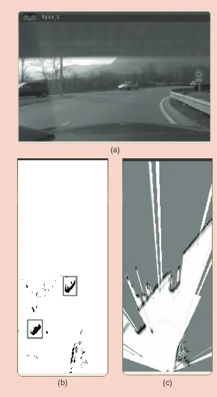
Figure 7. The MD results of two cars. (a) Driving scenario, (b) input fused grid, and (c) resulting motion grid and the noise is due to bushes along the road. (Photos courtesy of INRIA.)

(b) (c)

(a)

Results

Motion Detection

Some results of the MD module are shown in Figures 7 and 8, (rectangles around the objects are drawn manually to highlight them). As expected, the moving objects are prop-erly detected. For example, Figure 7 shows correct MD in a scenario with two cars. The car moving around a round-about in Figure 8 has also been successfully detected. Some noise is also visible on the results, mainly due to two causes: 1) localization errors along with the circular motion model may result in some errors in the estimation of the motion and 2) the decision function is too rough for taking correct decisions in every situation (especially for the regions having nonfixed objects like bushes and grass). The results would benefit from replacing this function by a probabilistic model.

Integration with FCTA

The following statistics, with a data set of about 13 min of driving on open roads, give an insight into the improvements gained with our new implementation. When the MD

mod-ule is not used, 22,303 moving objects (not tracks) in total are detected. The activation of the MD module, with all other parameters being equal, detects 4,796 moving objects in all frames. This example shows the advantage of the MD mod-ule because it allows us to remove most of the false moving objects while leaving most of the true dynamic objects. When considering tracks and not only detections, the results are also promising, as shown on Table 1.

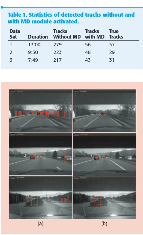
Some qualitative FCTA tracking results with and without MD module activated (with all other parameters being same) are also shown in Figure 9. Red rectangles are the detected tracks by FCTA in the depicted scenarios. We clearly see that most of the false positives have been removed.

Computation Time

All the components of the method are designed to be imple-mented on GPU with highly parallel processing. The mea-sured average computation time for each module is:

● multilayer fusion (GPU): 8 ms ● BOF update (GPU): 10 ms ● MD (CPU): 2.6 ms ● FCTA (CPU): 0.34 ms.

Thanks to the GPU implementation, the two first stages of the approach can work in real time. As expected, the MD module is fast despite the

CPU implementation. We hope to obtain an impor-tant gain from the GPU implementation. In addi-tion, this module allows us to significantly reduce the computation time of the FCTA by reducing the number of tracking hypotheses. As an exam-ple, for the same scene processed without and

with the MD module, the FCTA computation time is 0.5 and 0.34 ms, respectively.

Conclusions and Future Work

In this article, we have presented our current implementation of the BOF framework for dynamic environment monitoring. Compared with the previous implementation, we added two modules, which are well suited for the intelligent vehicle appli-cation. First, we propose a new approach for fusing the infor-mation from multiple layers of laser scanners, and computing the corresponding occupancy grid. Then, a fast technique to find moving objects from this grid data is proposed. The pre-sented technique does not require users to perform complete SLAM to detected moving objects, but uses grid data along with odometer/IMU information to transfer occupancy infor-mation between two consecutive grids.We have also presented its integration with BOF and FCTA. We have seen that, after this integration, we were able to remove a significant part of the detections resulting from the static environment.

(a) (b)

Figure 9. An example of tracking results for each scenario. (a) FCTA results without MD module activated and (b) with MD module activated. (Photos courtesy of INRIA.)

Table 1. Statistics of detected tracks without and with MD module activated.

Data

Set Duration

Tracks Without MD

Tracks with MD

True Tracks

1 13:00 279 56 37

2 9:30 223 48 29

3 7:49 217 43 31

Each layer can be used

to compute an occupancy

grid using the classical

range finder probabilistic

In the future, we plan to change the ad hoc decision module that is currently based on occupied and free counter values to a more formal probabilistic function that also takes into account the uncertainty effects on the neighboring cells to accommodate the localization errors. We also plan to implement multiple motion models to track moving objects with more accuracy and over longer periods of time.

Acknowledgments

This work was jointly supported by INRIA Grenoble Rhône-Alpes, Toyota Motor Europe, and the project “Prefect” from the IRT “Nano Elec” (A French Research and Innovation Project operated by the CEA and supported by the French Research Agency ANR). The authors would like to thank Dr. Dizan Vasquez and Dr. Trung Dung Vu for their technical support and fruitful suggestions.

References

[1] C. Laugier, I. Paromtchik, M. Perrollaz, M. Yong, J. Yoder, C. Tay, K. Mekh-nacha, and A. Negre, “Probabilistic analysis of dynamic scenes and collision risks assessment to improve driving safety,” IEEE Int. Transp. Syst. Mag., vol. 3, no. 4, pp. 4–19, 2011.

[2] R. Jain, W. N. Martin, and J. K. Aggarwal, “Segmentation through the detection of changes due to motion,” Comput. Graph. Image Process., vol. 11, no. 1, pp. 13–34, Sept. 1979.

[3] Z. Zhang, “Iterative point matching for registration of free-form curves and surfaces,” Int. J. Comput. Vis., vol. 13, no. 2, pp. 119–152, 1994.

[4] D. Li, “Moving objects detection by block comparison,” in Proc. IEEE Int. Conf. Electronics, Circuits Systems, 2000, vol. 1, pp. 341–344.

[5] S. Taleghani, S. Aslani, and S. Shiry. (2009). Robust Moving Object Detec-tion from a Moving Video Camera using Neural Network and Kalman Filter. Berlin Heidelberg, Germany: Springer-Verlag, pp. 638–648. [Online]. Avail-able: http://dl.acm.org/citation.cfm?id=1575210.1575268

[6] C.-C. Wang, C. Thorpe, and S. Thrun, “Online simultaneous localization and mapping with detection and tracking of moving objects: Theory and results from a ground vehicle in crowded urban areas,” in Proc. IEEE Int. Conf. Robot. Automation, Taipei, Taiwan, 2003, vol. 1, pp. 842–849.

[7] T.-D. Vu, J. Burlet, and O. Aycard. (2011). Grid-based localization and local mapping with moving object detection and tracking. Inform. Fusion [Online]. 12(1), pp. 58–69. Available: http://www.sciencedirect.com/science/article/pii/ S1566253510000187

[8] A. Petrovskaya and S. Thrun, “Model based vehicle detection and tracking for autonomous urban driving,” Auton. Robot., vol. 26, no. 2, pp. 123–139, 2009. [9] T.-D. Vu and O. Aycard, “Laser-based detection and tracking moving object using data-driven Markov chain Monte Carlo,” in Proc. IEEE Int. Conf. Robot. Automation, Kobe, Japan, May 2009, pp. 3800–3806.

[10] J. Moras, V. Cherfaoui, and P. Bonnifait. (2011, June 5–9). Moving objects detection by conflict analysis in evidential grids. Presented at IEEE Intelligent Vehicles Symp., Baden-Baden, Allemagne, pp. 1120–1125. [Online]. Available: http://hal.archives-ouvertes.fr/hal-00615304/en/

[11] J. Moras, V. Cherfaoui, and P. Bonnifait. (2011, May 9–13). Credibilist occupancy grids for vehicle perception in dynamic environments. Presented at

IEEE Int. Conf. Robotics Automation, Shanghai, China, pp. 84–89. [Online]. Available: http://hal.archives-ouvertes.fr/hal-00615303/en/

[12] R. Danescu, F. Oniga, and S. Nedevschi, “Modeling and tracking the driv-ing environment with particle-based occupancy grid,” IEEE Trans. Intell. Transp. Syst., vol. 12, no. 4, pp. 1331–1342, 2011.

[13] A. Elfes, “Occupancy grids: A stochastic spatial representation for active robot perception,” in Proc. 6th Conf. Annu. Conf. Uncertainty Artificial Intelli-gence, New York, 1990, pp. 136–146.

[14] A. Petrovskaya, M. Perrollaz, L. Oliveira, L. Spinello, R. Triebel, A. Makris, J.-D. Yoder, C. Laugier, U. Nunes, and P. Bessiere, “Awareness of road scene participants for autonomous driving,” in Handbook of Intelligent Vehi-cles. New York: Springer-Verlag, 2011.

[15] C. Tay, K. Mekhnacha, C. Chen, M. Yguel, and C. Laugier, “An efficient formulation of the Bayesian occupation filter for target tracking in dynamic environments,” Int. J. Auton. Veh., vol. T6, nos. 1–2, pp. 155–171, 2007. [16] C. Coué, C. Pradalier, C. Laugier, T. Fraichard, and P. Bessiere, “Bayesian occupancy filtering for multitarget tracking: An automotive application,” Int. J. Robot. Res., vol. 25, no. 1, pp. 19–30, Jan. 2006.

[17] K. Mekhnacha, Y. Mao, D. Raulo, and C. Laugier, “Bayesian occupancy fil-ter based ‘Fast Clusfil-tering-Tracking’ algorithm,” in Proc. IEEE/RSJ Int. Conf. Intelligent Robots Systems, Nice, France, 2008.

[18] T. Gindele, S. Brechtel, J. Schroder, and R. Dillmann, “Bayesian Occu-pancy grid Filter for dynamic environments using prior map knowledge,” in

Proc. IEEE Intelligent Vehicles Symp., Karlsruhe, Germany, 2009, pp. 669–676. [19] S. Thrun, W. Burgard, and D. Fox. (2005, Aug.). Probabilistic Robotics

(Intelligent Robotics and Autonomous Agents series). Cambridge, MA: MIT Press. [On line]. Ava i lable: ht tp://w w w.a ma zon.com/exec/obidos/ redirect?tag=citeulike07-20&path=ASIN/0262201623

[20] J. D. Adarve, M. Perrollaz, A. Makris, and C. Laugier, “Computing occu-pancy grids from multiple sensors using linear opinion pools,” in Proc. IEEE Int. Conf. Robotics Automation, St. Paul, MN, May 2012, pp. 4074–4079. [21] M. H. DeGroot. (1974). Reaching a consensus. J. Amer. Stat. Assoc.

[Online]. 69(345), pp. 118–121. Available: http://www.jstor.org/stable/2285509 [22] C. Coué, “Modèle bayésien pour l’analyse multimodale d’environnements dynamiques et encombrés: Application à l’ assitance à la conduite en milieu urbain,” Ph.D. dissertation, Dept. Comput. Sci., INPG, Natl. Polyt. Inst. Grenoble, 2003.

[23] Q. Baig and O. Aycard, “Improving moving objects tracking using road model for laser data,” in Proc. IEEE Intelligent Vehicles Symp., Alcala de Hena-res, Spain, June 3–7, 2012, pp. 790–795.

Qadeer Baig, INRIA Grenoble Rhône-Alpes, Grenoble, France. E-mail: qadeer.baig@gmail.com.

Mathias Perrollaz, INRIA Grenoble Rhône-Alpes, Grenoble, France. E-mail: mathias.perrollaz@inrialpes.fr; mperrollaz@ gmail.com.