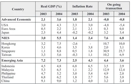
1. INTRODUCTION estimate in 2004 happened in Malaysia for 6,5 %, Economic growth is essential and needed while for Thailand, Philippines and Indonesia is because without it there is no improvement in estimated to reach 6,2;5,2 and 4,6 percent. This prosperity, job opportunity, productivity, and explanation can be seen in Table 1.1
income distribution. Economic growth is also From the Table 1.1, it can be seen that needed to prepare economy to the next progress. Indonesia economic growth estimate in 2004 is Indicator of economic growth is GDP explained still the lowest compared to neighboring by the differences between certain GDP with countries. It's not different as in 2003.
previous year GDP. GDP is goods value and In that context, one of economic factors can service produced in a country at a certain year leverage GDP growth or RGDP in a region and using production factors either residents' shows responsive economic policies to dynamic belonging or non-residents' belonging residing in economic development is investment. Economy the country. GDP can be measured either is developed when the total of goods production according market price or current price and fixed output and service availability in a certain year is price or constant price. higher than previous year's. In order to economy GDP growth in national level and GDP in can be developed, stock market must be added. regional level are important to reduction poverty, Additional capital good stock can be done unemployment, and increase residents' income. through investment. Investment invested is Thus, many policies and developments to hoped to improve output and input demand so it improve GDP growth and or GDP growth can affect revenue increase and expansion of job including economic growth indicators, economic opportunities which finally can boost economic structure become more productive, job growth. Creating investment in a country is opportunities expansion, improving income per essential to reach society prosperity. However, capita, and enhancement of development investment cannot happen by itself. Investment, distribution become important and has strategic especially private sector can only happen if value for Indonesia revival after stricken by many investors feel secure to invest their capital in prolonged crisis. another word investors will invest in a country if While for emerging market, including the condition of investment in the country is ASEAN-4 groups, the highest world growth conducive.
ANALYSIS OF THE INFLUENCE OF GOVERNMENT INVESTMENT, GROSS
DOMESTIC PRODUCT, REAL INTEREST RATES, AND THE GOVERNMENT'S
POLICY OF INVESTMENT TO PRIVATE INVESTMENT REALIZATION IN
INDONESIA FROM 1972 TO 2005
Vissia Dewi Haptari
Pusat Pendidikan dan Pelatihan Pajak E-mail: vissia_dh1@yahoo.com
ABSTRACT
This study tests the joint effects of Government Investment, Gross Domestic Product (GDP), Real Interest Rates, and Government's Policy on realization of private investment in Indonesia from 1972 until 2005. Government investment, the level of GDP and real interest rate directly have causality relationship with private investment, meaning every change in government investment, the level of GDP and real interest rate will cause positive change to private investment. On the other hand, the level of real interest rate does not have significant effect on investment, meaning the level of interest rate is not the only main cause, there are some other factors such as: inefficient institution condition which can be seen from complexity of rules, legal compliance system, and political stability.
Effort to increase investment become Three main complains from investors are important and urgent because reality shows that inefficient government, inadequate infrastructure capital investment especially foreign investment and complicated taxation regulation.
in Indonesia decreases. As written on newspaper, Exemption of tax income between 2-15 Indonesia Business (Monday, June 12, 2006), years has already given by ASEAN countries Indonesia position is faced to bad impression of (Malaysia, 5-15 years; Singapore, 5-10 years; International world. Reports from international Thailand, 5-8 years; Philippine,0-8 years; institution stated Indonesia is not a good place to Brunei, 2-5 years and China, 2-5 years), while invest. The image can decrease investment in Indonesia since 1984 has not been giving such Indonesia. The decline of investment in policy. Exemption or reducing of tax income has Indonesia can be seen in World Economic Forum also been given to the investors conducting report which declared that in 1999 investment research and development just like in Singapore th and Malaysia (Tang, 1993, p 161). This easiness competitiveness in Indonesia is at the 37 rank,
th has stimulated investors to invest their capital in and then became 44 in 2000. In 2001, Indonesia
th th the countries.
rank dropped to 49 and dropped again to 69 and
nd Compared to countries within East Asia and in 2002 until 2003 dropped again to 72 . As a
Asia Pacific, only Indonesia which has negative comparison in ASEAN level, Indonesia
Direct Foreign Investment (DFI). As a picture, in competitiveness kept going down under
th th 2003 net DFI flow in Indonesia was still negative Vietnam's which was at 60 in 2003 and 56 in
th nd (US$ 597 million). Besides that, DFI 2002 and Philippines at 66 in 2003 and 62 in
th contribution to Gross Fixed Capital Formation 2002. Indonesia position dropped from 69 in
th (GFCF) was still negative. In 2003, DFI
2004 became 74 in 2005. In improving
contribution to (GFCF) was -1,8 percent. The investment condition, there is no significant
condition was clarified by comparing DFI effort. In foreign perspective, business condition
Potential Index rank and DFI Performance in Indonesia in 2005 was getting bad. This can be
Index's as seen in Table 1.2. seen from Public Institution Index of Indonesia
th th
which fallen sharply from 68 to 89 in 2005.
Country Real GDP (%) Inflation Rate
On going transaction
2003 2004 2003 2004 2003 2004
Advanced Economic 2,1 3,6 1,8 2,1 -0,8 -0,8
USA
Emerging Asia 7,2 7,3 2,5 4,3 4,4 3,6
Indonesia
Source: World Economic Outlook September 2004 – IMF Table 1.1
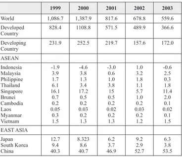
Study that has been done by The World Bank Table 1.3 shows between period 1986-1991 shows that DFI in ASEAN is fluctuated, except ratio DFI to GFCF in Indonesia was 2.4 percent Singapore, the best place for foreign investors. and was the lowest in ASEAN countries, while Overview about the condition can be seen in table ratio GFCF to GDP was 33.4 percent. It indicates 1.3 about ratio DFI to GFCF in ASEAN countries, that foreign investors are likely to invest their 1971-1991 in percent. capital in Singapore, Malaysia or Thailand
Table 1.2
Development of regional and global DFI flow (US$ Billion)
1999 2000 2001 2002 2003
World 1,086.7 1,387.9 817.6 678.8 559.6
Developed
Source: World Investment Report 2004 – UNCTAD
Description: number in parenthesis shows ratio GFCF to GDP Table 1.3
Ratio DFI to GFCF in ASEAN countries, years of 1971-1991 (in percent)
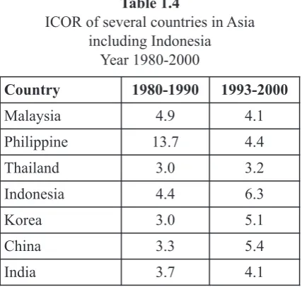
instead of Indonesia. First, investment by private through either The decline of Indonesia competitiveness if foreign capital investment or domestic capital compared with other countries is as a reflection of investment. Second, investment capital by the decline of investors' interest and trust toward government either through Government Budget investment opportunities in Indonesia. One of or Regional Government Budget. In reaching important issues highlighted in giving rating to economic growth, the most important condition investment in a certain country is through value is improving investment either by private or by indicator COR (Capital-Output Ratio) or ICOR government. Private investment to be a good (Incremental Capital-Output Ratio) which choice is DFI because it can improve technology, reflects efficiency level in either economic bring greater cash flow, have high skill, dominate financing or non-economic financing of international market, have access to international investment. It means investment in certain market. Actually, Indonesia has a potential to country needs low financing or high financing improve investment especially DFI.
can be seen by comparing ICOR indicator in a The decline of investment in Indonesia is a certain country. From this following data can be condition that does not stand alone meaning there seen ICOR in Indonesia compared to other are some correlated factors influencing the countries in Asia (Table 1.4) investment. Based on research conducted by World Bank there are some aspects influencing investment in a certain country which is how the country do the reform to strengthen business activities. From the research, Indonesia is still not the category conducted the reform.
From the previous overview, it can be seen that economic growth is still lower than other countries. In terms of investment, private investment in Indonesia is still not optimum. Seeing the condition, private investment become attractive to be observed and the condition can be observed more through creating investment indicators and economic variable namely government policy such as real interest rate, government investment, GDP, and the passing of policy in investment by the government. These are important things that have to be paid attention in describing the topic taken:
1. In reaching economic growth, the most Data above shows that in period 1980-1990 important condition is by improving ICOR in Indonesia was still relatively small, 4.4, investment either by government or private. even smaller that Malaysia, 4.9. The highest ICOR 2. Investment in Indonesia has shown is by Philippine, 13.7 percent. This coefficient improvement since monetary crisis in 1998, shows that in Philippine in 1980-1990, to add but the improvement has not maximized national output 1 unit needs additional capital because it still has the potential to be
13.7 units. improved. Since many factors have taken
However, in period 1993-2000, ICOR in part, so it is necessary to examine the factors. Indonesia seemed to be the highest compared to Based on the introduction, the issues to be other countries in Asia, 6.3. It showed that discussed in this study are:
efficiency in Indonesia was low. Low efficiency 1. How big the influence of government level would not attract foreign investors. investment to private investment?
Therefore, investment in Indonesia could not 2. How big the influence of GDP to private
compete with other countries. investment?
There are two kinds of investment offender. 3. How big the influence of real interest rate to Table 1.4
ICOR of several countries in Asia including Indonesia
Year 1980-2000
Country 1980-1990 1993-2000
Malaysia 4.9 4.1
Philippine 13.7 4.4
Thailand 3.0 3.2
Indonesia 4.4 6.3
Korea 3.0 5.1
China 3.3 5.4
India 3.7 4.1
private investment? Investment (I) is national income function (Yd), 4. How big the joint influence of government so it can be formulated as follows (Suparmoko,
investment, GDP, real interest rate to private BPFE;1990)
investment? I : F (Yd)
5. Is government policy in October 1993 I : IO + h Yd with Yd is national income influences private investment? I : investment
H : investment willingness
IO : investment spending that is not depend Theory, Former research, Hypothesis and on income (autonomous to investment) Methodology
C. Relationship between real interest rate
Theory with investment
A. Factors in Investment determination In Classical-Neo investment analysis, the Investment can be divided in to two, physical important thing emphasized in analyzing investment investment and financial investment. In terms of is real interest rate not nominal interest rate and economic analysis, physical investment is preferred. can be calculate with: Rs = rn – pe, with Rs is real To meet the expectation, there are some interest rate, rn is nominal interest and pe is conditions affecting investment determination inflation rate. Empirical study conducted by namely: National income, in this case, GDP, real Ficker shows that real interest rate is likely to be interest rate, government investment, and constant in a long term. In macro economy, relation-implementation of government policy in investment. ship of planned investment is depend on interest
rate r, in equation as follows: I = I(r). Relationship B. R e l a t i o n s h i p b e t w e e n G D P a n d between investment and interest rate is also
Investment described in Keynes theory about marginal
GDP is used to examine production level of a efficiency of investment showing that there is a country, it is calculation of every sector. Sector negative relationship between interest rate and contribution is role given by every sector to GDP. investment, high interest rate will reduce The calculation of GDP has some approach, investment and vice versa.
through production, income, and spending. In a
national economic balance, production value has D. Relationship between Government and to be equal with spending value. Economic indicator Private Investment
from spending is described with equation: GDP= Relationship between Government and C+ I + G (X - M). GDP is the sum of household Private Investment is described by Schmidt and consumption, government consumption, Muller in their research in 1991, In case of investment, and export subtracted by import. All Morocco, government investment can affect investment component has important role on private investment by competing in scarcity of economic growth and labor productivity physical and financial source. Real example of improvement. Capital stock is essential in this condition in developing country is when continuous economic growth (Solow, 1961) government create a barrier to private sector to Relationship between income and investment enter industry in order to protect state-owned spending is positive meaning if income increases, enterprises (ikhsan and Basri 1991, 365)
investment spending increases as well. On the
other hand, if income decreases, investment Several Former Research
Model (PAM), the result is all variables studied investment decision, and the meanwhile, interest have significant roles with trust level about 95%- rate cannot be separated from inflation. In 99%, researcher said that government need to September 2004, 3-month-interest rate and 12 make effort consistently and careful in month-deposit reach 7.31 percent and 7, 27 determining policy about investment. (Ika percent. While interest rate for rupiah loan for Anggia S: 2007). capital need and investment reach 13.80 and Another research is about the influence of 14.33 percent. Domestic interest rate development rate interest, exchange rate, export tax as during 2004 is lower than that of 2003 (Indonesia variables that affect private investment and non- Financial Economics Statistic - Bank of Indonesia). oil export and the effects on economic growth in In conclusion, if monetary authority reduces the Indonesia 1991-2003. Using description analysis amount of money through banking credit for method and analysis technique of correlation and private sector, real interest rate will increase. regression. The result showed that interest rate Consumption and investment will decrease. As a cannot predict but it has positive influence to result aggregate demand will decrease and this private investment, exchange rate can predict but causes declining of price rate and national output. it has positive influence to non-oil export. While Real interest rate used in the research is interest private investment influence is bigger than non- rate of 3 month-deposit. Election of the real oil export to economic growth (Bambang interest rate is based on the value of 3-month-Wijakmoko;2004) deposit interest rate is generally between saving
interest rate and loan interest rate. Also there are
Hypothesis many economic research use this variable.
Based on a problem and purpose, the The development of real interest rate of 3-hypothesis of this research is it is presumably that months-deposit between the year of 1976 until there is significant influences of factors affecting 2006 showed fluctuation, the highest value was private investment namely, real interest rate, 40% in 1998 and declined at 6.71% in 2004. In government investment rate, GDP, and influence 2005, rose again at 11.75%. The development of of policy implementation in investment. real interest rate of 3-months-deposit can be seen
in table 4.1 as follows: Method
In this research, used method is experimental quasi to explain causality between one or more other variables and also to clarify hypothesis. Investment as dependent variable, and government investment, GDP, real interest rate, and government policy implementation in investment as an independent variable. Data collection technique is by collecting official publications of Ministry of Finance, Central Bureau of Statistics, Bank of Indonesia, Capital Investment Coordinating Board and NGO institutions either national or International level. The data is a series of annual data from 1972 – 2005. Another technique is literature review from certain literatures, documents, journals, and other relevant reference materials. Analysis technique used is simple and multiple correlation analysis using data processing software, e-views.
Data Description 1. Real interest rate
Real interest rate is a cost element deciding
Table 4.2
Development of GDP year 1972 – 2005 based on constant price year of 2000
Year GDP (Billion Rp) Year GDP (Billion Rp)
1972 6,080.70 1989 200,568.60
1973 8,831.00 1990 234,654.60
1974 14,002.10 1991 2273,439.50
1975 16,531.80 1992 311,778.90
1976 20,224.80 1993 362,325.50
1977 24,859.00 1994 419,945.80
1978 29,743.00 1995 499,375.80
1979 41,877.50 1996 585,133.90
1980 59,426.30 1997 689,650.60
1981 70,647.50 1998 1,050,089.90
1982 77,624.50 1999 1,208,278.00
1983 93,122.70 2000 1,389,769.00
1984 107,833.60 2001 1,684,281.00
1985 116,329.50 2002 1,897,800.00
1986 123,186.50 2003 2,086,758.00
1987 149,740.70 2004 2,273,142.00
1988 170,480.70 2005 2,729.708.00
Year
Government
Investment
Year
Government
Investment
1972
165.10
1989
10,932.30
1973
246.30
1990
13,106.50
1974
907.90
1991
17,148.70
1975
1,049.90
1992
19,965.90
1976
957.20
1993
22,602.30
1977
1,029.60
1994
20,438.20
1978
1,117.80
1995
13,897.90
1979
2,123.60
1996
27,965.50
1980
3,423.00
1997
37,398.20
1981
6,313.20
1998
40,412.50
1982
6,633.20
1999
31,913.60
1983
7,538.40
2000
34,149.10
1984
3,412.50
2001
44,500.40
1985
9,316.30
2002
50,636.20
1986
6,890.10
2003
69,596.20
1987
8,727.50
2004
71,900.00
1988
9,703.10
2005
100,000.00
Table 4.3
2. Gross Domestic Product duty and additional customs duty, and Economic growth always becomes central simplification of import regulation is to issue in development matter, inflation and improve industrial efficiency and to develop payment balance. The analysis of economic downstream industries and supporting growth cannot be separated from the calculation industries of export to raise non-oil export of GDP because basically, calculating economic and to enhance job opportunities and finally growth is calculating how many GDP of a certain to anticipate Uruguay round. With regard to country. Central Bureau of Statistic of Indonesia competitiveness of goods that have been uses basic year of 2000. This value is used to produced within a country, there have been calculate GDP based on constant price by using taken various steps such as: fare reducing goods and service value at that year to eliminate and elimination and Import regulation the influence of price changes so the changes is changes.
only caused by real changes of output. The 3) Capital investment
development of GDP in Indonesia during Share ownership requirement in foreign research period can be seen in Table 4.2. capital investment has been refined to encourage foreign capital investment in
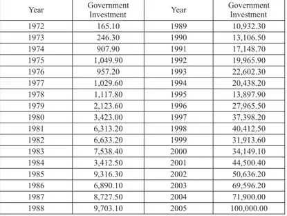
3. Government Investment developing their capital.
The purpose of government investment is to a. Outside of the bounded area:
improve society welfare. So, government ~ 100% foreign capital investment investment is social investment because with minimum capital of $50 generally investment spending is used to gain million, share transfer at 51% in 20 constant social capital or social overhead capital years, started at after 10 years such as: highway, harbor and irrigation, school, company has been operated hospital and dam construction. The development commercially.
of government investment in Indonesia during ~ It is possible for 100% foreign research period can be seen in Table 4.3. capital investment with minimum capital of $2 million on condition
4. Government Investment Policy that: the company produces
a. Policy Package October 23, 1993 auxiliary-raw materials, semi-Rapid changes in various parts of the world finished materials or other have spurred competition in capital investment components to fulfill other and trading between nations. In accordance with companies need. The purpose of demands of the development, it is necessary to this policy is to attract relocation improve national economic competitiveness such planning from developed countries as: simplification of the various licensing, and to enhance supporting procedures in capital investment, ease of goods industries.
flow, reducing of import duty and simplification b. Inside of the bounded area:
of import commerce. ~ Maximum export that can be
Government has established a set of entered in domestic market is 25%. deregulation and de-bureaucratization in various 4) Licensing
fields: Licensing procedures of land reserve,
1) Export and Import location license and building permit are Deregulation in export and import fields simplified.
is an ease of customs, taxation, and import 5) Farmation
commerce for EPTE goods mobilization, ~ Allowed to import registered finished bonded zone and customs area. The purpose drugs including the drugs not produced of the deregulation is to improve domestically.
attractiveness for investor especially in ~ I m p o r t c a n b e c o n d u c t i n g b y improving non-oil import. pharmaceutical factories, seller or drug
2) Fare and Import regulation store.
contracts between pharmaceutical of infrastructure 2006 and policy package of factories. investment. The policy package of infrastructure ~ Environmental Impact assessment 2006 includes four main policies: Strategic ~ Simplification of terms of reference of policy frame work across sectors, sectoral policy environmental impact assessment in transportation, regional government role in ~ Types of activities required environmental five policies related to regional owned impact assessment set by Ministers or enterprises and project transactions of Head of environmental impact control infrastructure development.
agency after considering arguments and
recommendation from the companies. d. Presidential Instruction number 6 year of 2007
b. Incentive package October 1, 2005 Presidential Instruction number 6 year of Incentive packages October 1, 2005 are an 2007 is a continuation of Presidential Instruction integral parts, implementation, and follow-up of number 3 year of 2006 which is about policy Policy package August31, 2005. The objectives package in improvement of investment to of this package is to empower economic based accelerate real sector development and to and to defense acceleration momentum of empower micro, small and middle business economic growth by improving competitiveness sector to increase economic growth including and attractiveness of investment to enlarge job improvement of investment, reformation of opportunities and to reducing poverty. financial sector, acceleration of infrastructure ~ Fiscal incentive package such as: changes of development, and empowerment of micro, small
value-added tax of primary product to non- and middle business sector.
taxable goods, deferment of non-tax 1) Development of Private Investment in revenues imposition for import and export Indonesia
transactions, enhancement of non-taxable An overview of the development of revenue and exemption of import duty. private investment in Indonesia can be seen ~ Regulation reformation in trading to through contribution and investment expedite goods flow, to increase competi- development in national revenue identity Y= tiveness and to protect domestic products. C+ I + G + X – M. Investment data is gross ~ Regulation reformation in transportation to domestic investment by either private reduce high-cost economy so that domestic investment or government investment. Table products can compete with international 4.4 shows investment in use of gross
market. domestic products based on prevailing price.
~ Changes of Presidential Instruction to From table 4.4, it can be seen that Gross stabilize farmer revenue as a result of rise in Domestic Product, according to
five-year-oil prices use is increased significantly. Investment
~ Direct cash subsidy started in October 1, contribution to Gross Domestic Product 2005 until the next three months, giving cash shows fluctuation as seen in the Table 4.5. at the amount of 100 thousands monthly to Private investment development in 15,5 million household with low income. Indonesia has been increased from year to year, except in period of after crisis (1999). c. Presidential Instruction number 3 year of Private investment development from 1971
2006 to 2005 based on constant price basic year of
Table 4.4 Calculation of National revenue (spending) based on prevailing price (billion)
Numb Types of use Year
1970 1975 1980 1985 1990 1995 2000 2005
1 Household
consumption
2,578 8,731 27,502 56,857 124,089 281,843 856,798 1,785,594
2 Government
consumption
293 1,253 4,688 10,893 17,572 35,584 90,779 224,980
3 Investment 455 2,571 9,485 21,779 61,623.20 129,217.50 275,881.20 599,795.20
4 Export 1,204 7,146 22,885 18,612 28,143 45,417 65,407 85,570
5 Import 1,102 5,409 14,242 12,552 23,028 40,627 40,365 57,550
6 Gross Domestic
Product
3,428 1,4292 50,318 95,589 208,399.2 451,434.5 1,248,500 2,638,389.2
Source: Ministry of finance, data from various years, processed
Table 4.5 Investment contribution to Gross Domestic Product
Year Gross Domestic
Product (billion) Investment ( billion) Contribution (%)
1970 3,428.00 455.00 13.27
1980 50,318.30 9,485.00 18.85
1990 208,399.20 61,623.20 26.26
2000 1,248,500 275,881.20 29.57
2005 2,638,389.20 599,795.20 22.73
Source: bank of Indonesia, processed
Year Private investment
(billion) Year
Private Investment (billion)
1972 910.10 1989 39,643.50
1973 1,269.30 1990 48,516.70
1974 1,346.60 1991 53,665.40
1975 2,176.60 1992 58,479.20
1976 3,063.70 1993 64,045.00
1977 3,771.00 1994 84,942.40
1978 4,742.10 1995 115,319.60
1979 6,287.70 1996 129,687.10
1980 8,477.20 1997 140,287.80
1981 8,181.80 1998 202,630.80
1982 10,263.00 1999 194,102.10
1983 14,025.50 2000 241,732.10
1984 18,891.60 2001 279,374.90
1985 15,458.70 2002 294,258.40
1986 20,559.90 2003 301,221.70
1987 25,588.20 2004 410,000.00
1988 31,061.90 2005 499,000.00
2) Investment in Indonesia problem in labor union (ISEI, 2006).
There are factors influencing investment Industrial partnership is one of crucial in Indonesia other than political and social points in economic competitiveness. stability, such as: economic stability, basic Although the total of strike does not increase infrastructure condition (electricity, significantly since reformation in 1998, the telecommunication and road and harbor risk of uncertainty caused by adversarial infrastructure), finance sector, labor market industrial partnership is the most essential including its issues, regulation and taxation, factor making attractiveness of Indonesia in bureaucracy, good governance including investment becomes lower.
corruption, consistency and certainty in Another serious problem is the government policies. Based on World Bank increasing of cost in doing business because report, there are four important factors: of regional autonomy. Budget constraints economic stability, corruption rate, bureau- and weak policy priority has caused pressure cracy, and certainty of economic policies. to improve tax revenue and regional Survey result from JETRO about retribution without taking into account the obstacles in business growth among Asian carrying capacity of the local and national countries shows different result. The biggest economy.
obstacle for investment in Indonesia is Recently, World Bank has published expensive labor wages and complicated reports called Doing Business 2007 and taxation. Survey conducted by IPEM in 2005 Doing Business 2008: “How to Reform” showed that cost to overcome labor problem about the ease of doing business in 2006. It th was 5% of annual production cost. Of the has placed Indonesia in the order of the135 600 respondents, 12.6% have experienced out of 175 countries in the world. This dispute in determining wages, 5.8% have condition is worse than before which is in the experienced problem related to labor social order of 131. Complete result of the report assurance, and 8.4% have experienced can be seen as follows:
st th
I. Starting a business in a 161 position in 2006 and 168 position in 2007
Reformation Criteria 2006 2007
Total of Procedure 12 12
Time needed (days) 97 105
Cost (% from income per capita) 86.7 80
Minimum capital (% from income per capita) 83.4 38.4
st th
II. Dealing with licenses in 131 position in 2006 and 99 position in 2007
Reformation Criteria 2006 2007
Total of Procedure 19 19
Time needed (days) 224 196
th rd
III. Employing workers in 140 position in 2006 and 153 in 2007
Reformation Criteria 2006 2007
Difficulty in determining of labor 61 72
Work hour limitation 20 0
Work termination 50 60
The average from three indexes 44 44
Overhead cost excluding wages charged 10 10
Severance costs to be paid 108 108
th st
IV. Registering property in 120 position in 2006 and 121 in 2007
Reformation Criteria
2006
2007
Total of procedure 7 7
Time needed (days) 42 42
Cost (% from property value) 10.5 10.5
rd th
V. Getting Credit in 83 position in 2006 and 68 in 2007
Reformation Criteria 2006 2007
Law enforcement 5 5
Transparency of credit information 2 3
Data provision by central bank about individual and organizational credit history
8.4 20.5
Data provision for company or organization about individual and organizational credit history
0.2 0.2
th st
VI. Protecting investors in 60 position in 2006 and 51 position in 2007
Reformation Criteria 2006 2007
Transaction information exposure by share holders 8 9 Accountability by the Board of Director for share
holders
5 5
Ease for share holders 3 3
Protection for investors 5.3 5.7
Reformation Criteria 2006 2007
Tax value (annual) 52 51
Time needed in tax payment (hour per annual) 576 266
Tax imposition (% from profit) 37.2 37.3
rd th
Hypothesis Testing and Results ~ Doing significance test of Z1 and Z2 by The first analysis step is testing the accuracy regressing each equation and adding Z1 to of equation through choosing the linear model or linear equation and Z2 to log equation. linear log using Mackinnon-White-Davidson ~ Selecting the right model is by seeing the (MWD) method. The procedure are as follows: significance of Z1 and Z2. If Z1 is significant ~ Doing estimation model of linear equation statistically, hypothesis is zero meaning the and linear log to get prediction value of F1 (= right model is linear will be rejected. On the I private - Res and F2 (=InY-Res02) other hand, if Z1 is insignificant, hypothesis ~ From step above, we can get value of Z1=In is zero, failed and rejected and so does with
F1-F2 and Z2=antilog F2-F1. Z2.
th st
VIII. Trading across borders in 60 position in 2006 and 41 in 2007
Reformation Criteria 2006 2007
Export document (total) 7 5
Time needed to export (days) 25 21
Export Cost (US $ per container) 546 667
Import Document (total) 10 6
Time needed to impor (days) 30 27
Import Cost (US $ per container) 675 623
th st
IX. Enforcing Contracts in 145 position in 2006 and 141 in 2007
Reformation Criteria 2006 2007
Total of Procedure 34 39
Time needed (days) 570 570
Cost (% from claim) 126.5 122.7
th
X. Closing a business in 136 position in 2006 and 2007
Reformation Criteria 2006 2007
Cost (% from estate) 5.5 5.5
Recovery rate, liabilities had to pay to creditors 18 18
The result of the calculation as below: Dependent variable: I private Method: Least Squares Date: 10/02/07 Time: 08:21 Sample (adjusted): 1983 2003
Included observations: 20 after adjustments
Variable Coefficient Std. Error t-Statistic Prob.
C 9852,757 7857, 163 1,253984 0,2304
Igovernment -0, 380193 0,622129 -0,611116 0,5509
GDP 0.144787 0,018608 7,781045 0,0000
Realinteresrate 9605,393 74525,89 0,128887 0,8993
Dummy 30701,30 9122,338 3,365508 0,0046
Z1 -3294,437 44247,92 -0,074454 0,9417
R-squared 0,989021 Mean dependent var 108544,1
Adjusted R-squared 0,985100 S.D dependent var 100006.4 S.e. of regression 12207.16 Akaike info criterion 21.90076
Sum squared resid 2.09E+09 Schwarz criterion 11.19948
Log likelihood -213.0076 F-statistic 252.2407
Durbin-Watson stat 1.207455 Prob (F-statistic) 0.000000
Dependent Variable: LOG (IPrivate) Method: Least Squares
Date: 10/02/07 Time: 08:22 Sample (Adjusted): 1972 2003
Included obeservations: 21 after adjustments
Variable Coefficient Std. Error t-Statistic Prob.
C -2.646629 0.476366 -5.555868 0.0001
LOG(IPrivate) -0.291224 0.095358 -3.054001 0.0080
LOG(GDP) 1.344573 0.108969 12.33905 0.0000
LOG(RealInterestrate) 0.231435 0.053383 4.335352 0.0006
DUMMY -0.053413 0.082935 -0.644030 0.5293
Z2 -1.57E-05 3.11E-06 -5.056288 0.0001
R-squared 0.996419 Mean dependent var 10.93051
Adjusted R-squared 0.995226 S.D dependent var 1.377423 S.E of regression 0.095174 Akaike info criterion -1.631261 Sum squared resid 0.135872 Schwarz criterion -1.332826
Log likelihood 23.12824 F-statistic 834.8320
Regression Results of both equation shows private investment. that linear model is more appropriate to explain 2. GDP Testing
private investment in Indonesia. It can be seen in t
~
Ho : â4 = 0, meaning GDP does not value at Z1 coefficient. Absolute t value is 0.074 affect significantly to private shows that Z1 is insignificant, because it is investment.smaller than t critical value in table at á=5% and
~
H1 : â4 ¹ 0 menaing GDP affects df=29 with the amount of 1.6999. In conclusion, significantly to private investment. Z1 is insignificant through t testing, so hypothesis 3. Real Interest rate Testing0 stated that appropriate regression function is
~
H0 : â3 = 0, meaning real interest linear model failed rejected. rate does not affect significantly toprivate investment.
Hypothesis testing
~
H1 : â3¹0, meaning real interest a. Testing Regression coefficient simultaneously rate affects significantly to private
Relationship among government investment, investment.
GDP, real interest rate and government 4. Implementation of government policy policy simultaneously with below hypothesis: Testing
H0 : â1Dt = â2 = â3 = â4 = 0 meaning real
~
H 0 : â 3 = 0 , m e a n i n g interest rate, government investment, GDPimplementation of government and government policy do not affect
policy does not affect significantly significantly to private investment.
to private investment. H1 : â1Dt = â2 = â3 = â4? 0 meaning real
~
H 1 : â 3 ¹0 , m e a n i n g interest rate, government investment, GDPimplementation of government and government policy affect significantly to
policy affects significantly to private investment.
private investment. b. Testing Regression coefficient partially
Hypothesis testing (rejected or accepted) 1. Government Investment testing
uses t table as single measurement and F table as
~
H0 : â3 = 0, meaning governmentmultiple measurement. If t/F value > t/F table, H0 investment does not affect
is rejected and H1 is accepted and if t/F value < t/F significantly to private investment.
table, H1 is accepted and H1 is rejected with trust ~ H1 : â3 ¹ 0, meaning government level 95% or á = 5%. Hypothesis testing uses
investment affects significantly to
Eviews program and the result is below:
Dependent Variable: IPRIVATE Method: Least Squares
Date: 10/02/07 Time: 11:51 Sample: 1972 2005
Included observations: 34
Variable Coefficient Std. Error t-Statistic Prob.
C -2393.374 3545.619 -0.675023 0.5050
GDP 0.127733 0.014019 9.111200 0.0000
IGOVERNMENT 1.141133 0.437508 2.608254 0.0142
REALINTERESTRATE -1.9525.85 20141.04 -0.969456 0.3403
DUMMY 14792.32 8318.100 1.778329 0.0858
R-squared 0.988750 Mean dependent var 98029.46
Adjusted R-squared 0.987198 S.D dependent var 129968.2 S.E of regression 14705.44 Akaike info criterion 22.16488
Sum squared resid 6.27E+09 Schwarz criterion 22.38934
Log likelihood -3371.8029 F-statistic 637.1746
R-squared value is 0.988 meaning private model, done by using Durbin Watson test, easiest investment variable can be explain by test and can be compared directly with statistical explanatory variable in a model: government value of Durbin Watson table. To know whether investment, GDP, interest rate and dummy with there is any deviation of autocorrelation model or amount 98.80%, while the residue is explained by not is by using position of Durbin Watson value other variables outside the proposed model. gotten from multiple regression calculation. This Analysis result shows that all independent step will test whether there is any mistake at t variables simultaneously affect the dependent period with disturbing mistake at previous period variable, shown by F-stat = 637.17, which is (t-1) in linear regression model.
bigger than F table at á 5% (4.29 is from k-1, n-k Autocorrelation emerges because successive = 5-1, 34 – 5) = 2.56. Individually, government observation from time to time related one investment variable has a positive and significant another. It is because residue is not free from one influence at á 1 and 5 % shown by t value = 9.111 observation to another. Given that there is an compared to t table (df = 29), 2.462 and 1.699 intercept (c) in this model and no lag variable in
respectively. independent variable, to detect whether there is
GDP variable also has a positive and any autocorrelation or not, Durbin – Watson (DW significant influence at á 1 and 5 % shown by t test) can be used. Criteria of decision making value = 2.608 compared to t table (df = 29), 2.462 related with autocorrelation presence are as and 1.699 respectively. In contrast, real interest follows:
rate variable does not affect private investment at 1. Area 0 < dw < dL, positive autocorrelation at á 5 % shown by t value = 0.969 which is smaller 2. Area dL < dw < dU, hesitation area than t table (df = 29) at 1.699. However, from the 3. Area dU < dw < 4 – dU, no autocorrelation sign test, there is a conformity with theory which 4. Area 4 – dU < dw < 4- dL, hesitation area can be shown from negative relationship between 5. Area 4 – dL < dw < 4, negative investment and interest rate. Dummy variable has autocorrelation
a positive and significant influence as well to From regression analysis can be seen that the private investment at á 5 % shown by t value = calculation shows Durbin Watson value at 1.782. 1.778 compared to t table (df = 29) 1.699. After consulted with Durbin Watson table where Based on testing above, It can be made a dL : 1.208 and dU : 1.728 (n+34 and df = 4) it can regression equation: IPrivate = C + 0.128 GDP + be concluded that dw value is at between 1.728 – 1.141 IGovernment – 0.19525.85 RInterestRate. 2.272, it shows that model has passed Next, to get regression line exactly near with the autocorrelation. Besides that, test can be done by data in order to get exact prediction, ordinary using Breusch-Godfrey Test (BG – test), least square (OLS) method was used and to calculating residual value first (Res) and the produce BLUE (Best Linier Unbiased value will be transformed in to lag variable Estimators) long term regression, classical test (Res_1), next BG test uses regressed model: assumption was used, such as: Res = a + b1 Igovernment + b2 GDP + b3
Output display shows that coefficient another, it is called homoscedasticity, and if it is parameter for residual lag 1 (res_1 or Res (- different, it is called heteroscedasticity. 1) gives significant probability at the amount Heteroscedasticity occurs as the effect of residual of 0.7013. This result confirms that that has no constant variant from one observation Hypothesis 0 failed rejected because to another. This research uses park test to detect significant probability values is bigger than the presence of heteroscedasticity by regressing
2
= á 5% or 0.05 meaning that there is no square residual log (µ t) as dependent variable, autocorrelation in a model. with independent variable: government investment, GDP, and real interest rate in
Heteroscedasticity Detection logarithm.
2 Heteroscedasticity symptom test to test This park method expresses that variance (s ) whether there is a difference in variance form one is the function of independent variables stated in
2
residual observation to another using auxiliary equation : o i = á Xi â. Next, the equation is 2
regression, residual value (ei) with other converted in logarithm Ln o I = á + â Ln Xi + vi. 2
independent variables (after equation is changed Because o I is generally unknown then it is with natural logarithm (Ln), next, hypothesis estimated by using residual Ut as a proxy then
2
testing is conducted with t - test, with certain trust equation becomes Ln U I as a dependent and degree (á) with freedom degree df (n-k), t-table independent variable, so regression equation
2
value can be determined. If t-test > t=table, there becomes: Ln U i = a + b1 X1 + b2 X2 + b3 X3 - b4 is a heteroscedasticity. In contrast, if the t-test > t- X4. If beta coefficient parameter in equation is table, there is no heteroscedasticity. significant statistically, then it shows that there is The purpose of this step is to test whether heteroscedasticity in a model estimated and vice there is any variant differences from one residual versa, if beta parameter is insignificant observation to another. If the residual observation statistically, then the assumptions of homos-variants is constant from one observation to cedasticity in the model is failed rejected.
Variable Coefficient Std. Error t-Statistic Prob.
C -113.6391 3784.779 -0.030025 0.9763
IGOVERNMENT -0.029999 0.465942 -0.064384 0.9491
GDP 0.001229 0.015028 0.081762 0.9354
REALINTERESTRATE -966.9488 20.923.00 -0.046215 0.9635
DUMMY -22.89916 8609.736 -0.002660 0.9979
RES (-1) 0.080620 0.207988 0.387619 0.7013
R-squared 0.005607 Mean dependent var -103.4027
Adjusted R-squared -0.178540 S.D dependent var 13985.77
S.E of regression 15183.03 Akaike info criterion 22.25671
Sum squared resid 6.22E+09 Schwarz criterion 22.52880
Log likelihood -361.2357 F-statistic 0.030450
Durbin-Watson stat 1.860007 Prob(F-statistic) 0.999485
Dependent variable : RES Method : Least Square Date : 10/02/07 Time : 07:53 Sample (adjusted): 1973 2005
2
Calculation shows that coefficient parameter determination coefficient (R ) is high, is insignificant for independent variable (because significant F statistics, but only a few sifnificancy of á > 0.05) then H0 stated that there independent variables which significantly is no heteroscedasticity in the model is failed affect dependent value through t test. From rejected. It can be concluded that there is data processing, it can be seen that this homoscedasticity in regression model or in symptom does not occur, because the another word there is no heteroscedasticity. calculation shows that determination
2
coefficient (R ) is high, significant F Multicollinearity Detection statistics, and most of independent variable This test intends to measure whether there is is significant, it can be concluded that there is a correlation among independent variable in no multicollinearity in the model.
regression model. The right regression model ~ To support test result, partial regression is should not contain correlation among its conducted by using auxiliary regression independent variables. The following ways are among independent variables and then
2 2 2
used to detect multicollinearity presence in a comparing R value with R main model. If R
model: is higher than main model, then it can be
~ In a simple way multicollinearity symptom confirmed that there is multicollinearity in can be known from long term regression partial regression.
r e s u l t b y s e e i n g t h e p r e s e n c e o f Result:
2 Dependent Variable: LOG (RES ) Method: Least Squares
Date: 10/02/07 Time: 22:06 Sample (adjusted): 1972 2003
Included observations: 21 after adjustments
Variable Coefficient Std. Error t-Statistic Prob.
C 12.20536 9.853354 1.238702 0.2333
LOG(IGOVERNMENT) -0.883060 1.596888 -0.552988 0.5879
LOG(GDP) 0.908447 1.778388 0.510826 0.6164
LOG(REALINTERESTRATE) -0.295624 1.103971 -0.267782 0.7923
DUMMY 1.797993 1.895074 0.948772 0.3568
R-squared 0.253090 Mean dependent var 16.90498
Adjusted R-squared 0.066362 S.D dependent var 2.461597
S.E of regression 2.378516 Akaike info criterion 4.775088
Sum squared resid 90.51744 Schwarz criterion 5.023783
Log likelihood -45.13842 F-statistic 1.355397
Dependent variable: I Government Method: Least Square
Date: 10/02/07 Time:22:18 Sample: 1972 2005
Included observations : 34
Variable Coefficient Std. Error t-Statistic Prob.
C 319.422 1359.418 2.353524 0.00253
GDP 0.029610 0.002236 13.24084 0.0000
REALINTERESTRATE 1222.148 8401.987 0.145459 0.8853
DUMMY 1828.230 3455.096 0.529140 0.6006
R-squared 0.940186 Mean dependent var 20474.03
Adjusted R-squared 0.934205 S.D dependent var 23924.02
S.E of regression 6136.649 Akaike info criterion 20.39208
Sum squared resid 1.13E+09 Schwarz criterion 20.57165
Log likelihood -342.6653 F-statistic 157.1854
Durbin-Watson stat 0.892805 Prob(F-statistic) 0.000000
Dependent variable: GDP Method: Least Square Date: 10/02/07 Time:22:20 Sample: 1972 2005
Included observations : 34
Variable Coefficient Std. Error t-Statistic Prob.
C -77418.39 43.958.05 -1.761188 0.0884
IGOVERNMENT 28.83754 2.177924 13.24084 0.0000
REALINTEREST RATE -53395.43 262115.8 -0.203709 0.8400
DUMMY 122502.0 105992.7 1.155759 0.2569
R-squared 0.942149 Mean dependent var 559624.7
Adjusted R-squared 0.9363364 S.D dependent var 759166.6
S.E of regression 191509.1 Akaike info criterion 27.27339
Sum squared resid 1.10E+12 Schwarz criterion 27.45296
Log likelihood -459.6476 F-statistic 162.8574
Dependent variable: Real Interest rate Method: Least Square
Date: 10/02/07 Time:22:21 Sample: 1972 2005
Included observations : 34
Variable Coefficient Std. Error t-Statistic Prob.
C -0.007606 0.032110 -0.236878 0.8144
IGOVERNMENT 5.77E-07 3.96E-06 0.145459 0.8853
GDP -2.59E-08 1.27E-07 -0.203709 0.8400
DUMMY 0.037493 0.075090 0.499307 0.6212
R-squared 0..013469 Mean dependent var 0.004059
Adjusted R-squared -0.085184 S.D dependent var 0.127963
S.E of regression 0.133302 Akaike info criterion -1.082273
Sum squared resid 0.533080 Schwarz criterion -0.902701
Log likelihood 22.39865 F-statistic 0.136527
Durbin-Watson stat 1.530913 Prob(F-statistic) 0.937442
Dependent variable: Dummy Method: Least Square Date: 10/02/07 Time:22:21 Sample: 1972 2005
Included observations : 34
Variable Coefficient Std. Error t-Statistic Prob.
C 0.083172 0.076327 1.089680 0.2845
IGOVERNMENT 5.06E-06 9.56E-06 0.529140 0.6006
GDP 3.48E-07 3.01E-07 1.155759 0.2569
REALINTERESTRATE 0.219820 0.440251 0.499307 0.6212
R-squared 0.610754 Mean dependent var 0.382353
Adjusted R-squared 0.571829 S.D dependent var 0.493270
S.E of regression 0.322770 Akaike info criterion 0.686378
Sum squared resid 3.125416 Schwarz criterion 0.865950
Log likelihood -7.668427 F-statistic 15.69070
Durbin-Watson stat 0.374464 Prob(F-statistic) 0.000003
2
Discussion of the result Auxiliary regression shows each R value is
Data used in the research is annual data such 0.940; 0.942; 0.013; 0.610. The values are
2 as private investment, real interest rate, smaller if compared with R in the main model
government investment and GDP from 1972 to (=0.988). Then it can be confirmed that there is no
Year Private Investment (Y)
Government
Investment GDP Real Interest Rate Dummy
1972 910.10 165.10 6,080.70 0.055 0
1973 1,269.30 246.30 8,831.00 -0.228 0
1974 1,346.60 907.90 14,002.10 -0.312 0
1975 2,176.60 1,049.90 16,531.80 -0.099 0
1976 3,063.70 957,20 20,224.80 -0.11 0
1977 3,771.00 1,029.60 24,859.00 -0.049 0
1978 4,742.10 1,117.80 29,743.40 -0.023 0
1979 6,287.70 2,123.60 41,877.50 -0.103 0
1980 8,447.20 3,423.00 59,426.30 -0.117 0
1981 8,181.80 6,313.20 70,647.50 -0.066 0
1982 10,263.00 6,633.00 77,624.50 -0.033 0
1983 14,025.50 7,538.40 93,122.70 0.036 0
1984 18,891.60 3,412.50 107,833.60 0.071 0
1985 15,458.70 9,316.30 116,329.50 0.106 0
1986 20,559.90 6,890.10 123,186.50 0.087 0
1987 25,588.20 8,727.50 149,740.70 0.084 0
1988 31,061.90 9,703.10 170,480.70 0.096 0
1989 39,643.50 10,932.30 200,568.60 0.108 0
1990 48,516.70 13,106.50 234,439.50 0.097 0
1991 53,665.40 17,148.70 311,778.90 0.141 0
1992 58,479.20 19,965.90 362,325.50 0.119 0
1993 64,065.00 22,602.303 419,945.80 0.049 1
1994 84,942.40 20,438.20 499,375.80 0.04 1
1995 115,319.60 13,897.00 585,133.90 0.074 1
1996 129,687.10 27,965.50 689,650.60 0.093 1
1997 140,287.80 37,398.20 689,650.60 0.092 1
1998 202,630.80 40,412.50 1,050.089.00 -0.376 1
1999 194,102.10 31,913.60 1,208.278.00 0.233 1
2000 241,732.10 34,149.10 1,389,769.00 0.031 1
2001 279,374.90 44,500.40 1,684,281.00 0.029 1
2002 294,258.40 50,636.20 1,897,800.00 0.052 1
2003 301,221.70 69,596.20 2,086,758.00 0.051 1
2004 410,000.00 71,900.000 2,273,142.00 0 1
Based on hypothesis testing and calculation, 14792.32 meaning policy change has caused then analysis among research variables are as an increase in private investment of
follows: 14792.32 billion.
a. All independent variables: government Based on above-mentioned analysis, it can be investment, GDP, real interest rate, described:
government policy simultaneously affect 1. Private investment as a variable in this dependent variable, private investment. This research has been influenced by many shows that all the government's policies, factors. It can be concluded that private fiscal policy, monetary policy, and income investment is positively influenced by have an effect on private investment. real interest rate, government investment, b. Based on individual calculation, relationship GDP, either individually or as a whole in
between government investment and private a causality relationship.
investment has a positive and significant 2. Government Investment in the form of effect, with government coefficient 1.411 government spending through its meaning 1 billion investment will cause spending budget which function to increase in private investment of 1.141 empower real sector, based on test, also billion. This shows that government can influence private investment. investment is usually in the provision of 3. GDP level in the form of economics infrastructure to encourage new private ability of a nation as a whole has
investment. positive influence to private investment
c. Based on individual calculation, relationship change.
between GDP and private investment has a 4. Real interest rate in the form of the positive and significant effect, with difference between income per capita in government coefficient 0.128 meaning 1 relationship with Domestic Purchasing billion investment will cause increase in Power, where society have high private investment of 0.128 billion. This purchasing power will support shows that with increasing GDP as state investment.
revenue can encourage private investment. 5. Real interest rate in the form of the d. Based on individual calculation, relationship difference between interest rate between real interest rate and private generally applicable with inflation rate, investment, it does not affect private individually, has no significant effect on investment. However, from sign conformity private investment. Thus, private test, there is a conformity with theory, it can investment has no sensitivity towards be seen in negative relationship between interest change meaning there is another investment and interest rate. Presumably, factor namely institutional condition. there are other variable more determining 6. Implementation of government policy, towards private investment during research in this case, policy set in 1993 has period, such as: security condition and significant influence on private investment deregulation policy. This is in investment because government policy accordance with concept of inelastic demand change can support investment curve where investment sensitivity is lower condition, for examples, simplification towards interest change. of licensing, procedures in capital e. Based on individual calculation, dummy investment, easiness in goods flow, variable, the influence of implementation of reduction of import duty, and simplifi-government policy in investment, it can be cation of import regulation.
seen that implementation of government policy, October 23, 1993 (October Package
1993) used as measurement in implemen- RECOMMENDATION
reformation of institution, and regulation of in Mankiw, Gregory N., 2000, Macroeconomics, investment. Moreover, to synergizing policy is Tranlated Nurmawan, Imam (2000) Teori
t h
also essential since inaction of policy implemen- Makro Ekonomi, 4 . Ed., Publisher tation is a root cause of lack of investment. Erlangga.
Maryatmo, R. 2004, “Dampak Moneter
REFERENCE Kebijakan Defisit Anggaran Pemerintah dan
Peranan Asa Nalar dalam Simulasi Model Bank Indonesia, Statistik Ekonomi Keuangan Makro-Ekonomi Indonesia (1983-2002:4) Indonesia,various edition, Jakarta “Buletin Ekonomi Moneter dan Perbankan,
page 297. Departemen Keuangan Indonesia RI, Nota
Keuangan dan Rancangan Anggaran Nachrowi, Djalal, Nacrowi dan Usman, Hardius Pendapatan dan Belanja Negara,various Usman, 2005, Penggunaan Teknik
edition, Jakarta Ekonometri, revised edition, Publisher Raja
Grafindo Persada. Dornbusch, et al. 2001, Macroeconomics,
translated Wibisono, Yusuf (2001) Teori Nugroho, Sulaiman Adi (2005), Analisis th
Makro Ekonomi , 8 . Ed., Publisher Media Investasi Di Indonesia serta Faktor-faktor
Global Edukasi. Ekonomi yang mempengaruhi, tahun
1979-2003, Yogyakarta, Sekolah Tinggi Ilmu Gujarati, Damodar N. 2003. Basic Econometric, Ekonomi.
th
4 . Ed. New York : Mc. Graw Hill
Nuryanto, Wahyu, 2005, “The Effect of International Edition.
Government Expenditure and Tax Policy on Economic Growth,” Jurnal Keuangan Gordon, Robert J. 1978. “Macroeconomics”. By
Publik, 3.(2). 45-55 Little Brown and Company, Canada.
Putong, Iskandar, 2007,”Economics, Pengantar Herderschee, H. 1993, Incentive for Exports: The
Mikro dan Makro, latest edition, Publisher Case of Thailand”, ASEAN Economic
Mitra Wacana Media, Jakarta. Bulletin, 9, hal 48-363.
Sukirno, Sadono 2004, Makro Ekonomi Teori I S E I 2 0 0 6 , “ R e k o m e n d a s i K e b i j a k a n
Pengantar, Raja Grafindo Perkasa, Jakarta. Pemerintah. Langkah-langkah Strategis
Pemulihan Ekonomi Indonesia”. Jakarta:
Supancana, Ida Bagus Rahmadi, 2006, Kerangka Ikatan Sarjana Ekonomi Indonesia.
Hukum Kebijakan Investasi Langsung di Indonesia, Bogor: Ghalia, Indonesia.
Kojima, R 1992, “The Growing Fiscal Authority of Provincial – Level Government in China”,
Tang, S.S.C. 1993, “The Legislative Framework The Developing Economics, 30, hal 315 –
for Direct Foreign Investment in ASEAN”, 326
ASEAN Economic Bulletin, 10 page 155-165.
Lukman, Rizal Affandi, 2006, lecture notes Seminar Kebijakan Ekonomi dan Industri
Todaro, Michael. 1994, Economic Development, Indonesia.
Longman. Terjemahan. Munandar Haris th Lembaga Penelitian Ekonomi IBII, 2004, Makro (2000), Pembangunan Ekonomi, 5 . Ed.
UNCTAD 2004, World Investment Report 2004, World Bank, Brief for The Consultative Group on New York & Geneva: UN Indonesia, 2006, Investing for Growth and
Recovery, World Bank, Jakarta. WEF 2004, The Global Competitivesness Report
2004-2005, Geneva: World Economic World Bank, 2006, Doing Business 2007, How to
Forum Reform, Comparing Regulation in 175
Economies, World Bank, Jakarta WEF 2005, The Global Competitivesness Report
2005-2006, Geneva: World Economic World Bank, 2007, Doing Business 2008, How to
Forum Reform, Comparing Regulation in 178
Economies, World Bank, Jakarta Widarjono, Agus, 2005, Ekonometrika Teori dan
Aplikasi, untuk Ekonomi dan BIsnis, Keputusan Presiden Nomor 29 tahun 2004 Ekonisia, Yogyakarta. tentang Penyelenggaraan Penanaman Modal Dalam Rangka Penanaman Modal Asing dan Widjaya, I.G. Rai,, 2005, Penanaman Modal, Penanaman Dalam Negeri Melalui Satu
Pedoman Prosedur Mendirikan dan Atap. Menjalankan Perusahaan dalam Rangka
PMA dan PMDN, Jakarta: Pradnya Paket Kebijakan 23 Oktober 1993, tentang
Paramita. Kebijakan Deregulasi di Bidang Ekspor
Impor, Tarif dan Tata Niaga Impor, Widodo, Suseno Triyanto, 1990, Indikator Penanaman Modal, Perijinan, Farmasi, dan
Ekonomi, Penerbit Kanisius, Yogyakarta. Amdal.
World Bank 2004, Executive Summary, “A Instruksi Presiden, Nomor 3 tahun 2006, tentang Raising of Investment in Indonesia, World Paket Kebijakan Perbaikan Iklim Investasi. Bank, Jakarta
Instruksi Presiden, Nomor 6 Tahun 2007 tentang World Bank 2005, Iklim Investasi yang Lebih Kebijakan Percepatan Pengembangan Baik bagi Setiap Orang, Laporan Sektor Riil dan Pemberdayaan Usaha Mikro, Pembangunan Dunia 2005, The World Bank, Kecil dan Menengah.