1
Variability of Soil Physical Properties in a Clay -Loam Soil and Its Implication on Soil 1
Management Practices 2
3
Samuel I. Haruna and Nsalambi V. Nkongolo* 4
Center of Excellence for Geospatial Information Sciences, Department of Agriculture and 5
Environmental Science, Lincoln University, Jefferson City, MO 65102-0029 6
7
*Corresponding author: [email protected] 8
9
10
11
12
13
14
15
16
17
18
19
20
21
22
2 Abstract
1
We assessed the spatial variability of soil physical properties in a clay- loam soil cropped to corn 2
and soybean. The study was conducted at Lincoln University in Jefferson City, Missouri. Soil 3
samples were taken at four depths: 0-10 cm, 10-20, 20-40 and 40-60 cm and were oven dried at 4
105oc for 72 hours. Bulk density (BDY), volumetric (VWC) and gravimetric (GWC) water 5
contents, volumetric air content (VAC), total pore space (TPS), air- filled (AFPS) and water-6
filled (WFPS) pore space, the gas diffusion coefficient (Diff) and the pore tortuosity factor (Tort) 7
were calculated. Results showed that in comparison to Depth 1, means for AFPS, Diff, TPS, and 8
VAC decreased in Depth 2. In opposite, BDY, Tort, VWC and WFPS increased in depth2. 9
Semivariogram analysis showed that GWC, VWC, BDY and TPS in depth 2 fitted to an 10
exponential variogram model. The range of spatial variability (Ao) for BDY, TPS, VAC, WFPS, 11
AFPS, Diff and Tort was the same (25.77 m) in depth 1 and 4, suggesting that these soil 12
properties can be sampled together at a same distance. The analysis also showed the presence of 13
a strong (≤ 25%) to weak (>75%) spatial dependence for soil physical properties. 14
15
Key Words: Spatial variability, physical properties, semivariogram, depth, clay- loam soil 16
17
18
19
20
21
22
3 1. Introduction
1
Characterizing the spatial variability and distribution of soil properties is important in predicting 2
the rates of ecosystem processes with respect to natural and anthropoge nic factors [1], and in 3
understanding how ecosystems and their services work [2]. In agriculture, studies of the effects 4
of land management on soil properties have shown that cultivation generally increases the 5
potential for soil degradation due to the breakdown of soil aggregates and the reduction of soil 6
cohesion, and thus a decrease in soil nutrient content [3, 4]. Cultivation, especially when 7
accompanied by tillage, have been reported to have significant effects on topsoil structure and 8
thus the ability of soil to fulfill essential soil functions and services in relation to root growth, gas 9
and water transport and organic matter turnover [5, 6, 7]. The physical properties of the soil are 10
affecting soil physical properties is human influence through agricultural practices of soil tillage, 14
crop rotation and cover cropping. Soil properties vary considerably under different crops, tillage 15
type and intensity, fertilizer types and application rates. Since this variability affects soil water 16
and nutrient content dynamics and other soil physical processes, knowledge of the spatial 17
variability of soil properties is therefore necessary. 18
To study the spatial distribution of soil properties, techniques such as classical statistics and 19
geostatistics that seek to show spatial and spatiotemporal variations have been widely applied [9, 20
10, 11]. Geostatistics provides the basis for interpolation and interpretation of the spatial 21
variability of soil properties [9, 12, 13, 14]. Information on soil spatial variability leads to better 22
4
sustainability of the soils, and thus increasing the precis ion of farming practices [1, 15]. A better 1
understanding of the spatial variability of soil properties would enable for refining agricultural 2
management practices by identifying sites where remediation and management is needed. This 3
promotes sustainable soil and land use, and also provides valuable base against which subsequent 4
future measurements can be proposed [14]. Despite its importance in agriculture, literature is 5
lacking on the variability of soil physical properties in central Missouri, especially at the lower 6
depths (30-60cm). The objective of this study, therefore, was to assess the spatial variability of 7
soil physical properties in a clay- loam soil field and determine how knowledge on this variability 8
can affect agricultural management practices. 9
10
2. Materials and methods 11
2.1 Experimental site 12
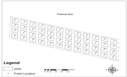
The study was conducted at Lincoln University‟s Freeman farm in Jefferson City, Missouri. The 13
geographic coordinates of the study site are 38058‟16”N latitude and 92010‟53”W longitude. 14
Prior to establishment in 2011, the farm was a 80.94 ha farm in the bottomland of the Missouri 15
river. It was mainly planted to corn and soybean, with conventional tillage (moldboard) for over 16
50 years. The soil type is mainly Waldron clay- loam (Fine, smectitic, calcareous, mesic Aeric 17
Fluvaquents). The study area is almost flat, with an average slope of 2%. The experimental field 18
(Fig. 1.) is a 4.05 ha field divided into three blocks (replicates) using complete randomized block 19
design. Each block of 1.35 ha contains 16 plots for a total of 48 plots. Each plot measured 12.2m 20
x 21.3m. Half (Twenty four) of the plots were planted to Corn (Zee mays) while the other half 21
was grown to Soybean (Glycine max). As part of the standard research protocol for the grant that 22
5
nitrogen, 67.25 kg/ha of phosphorus, and 89.67 kg/ha of potassium. Corn plots received 201.75 1
kg/ha of additional nitrogen in the form of urea. 2
3
2.2 Soil sampling 4
Cylindrical cores of 3.15 cm radius and 10 or 20 cm heights were used to collect soil samples in 5
were collected: 48 plots x 4 depths x 3 replicates (in each plots). To eliminate compaction that 9
sample; FWS), then oven dried at 105oC for 72 hrs. The weight was taken after oven drying (Dry 13
weight of Soil; DWS). Soil physical properties were calculated as follows: Soil bulk density 14
(BDY, g.cm-3) = DWS/V, where DWS is the dry weight of soil and V the volume of cylinder 15
(total volume of soil); Volumetric water content (VWC, cm3.cm-3) = (FWS-DWS)/V, with FWS 16
being the fresh weight of soil; Gravimetric water content (GWC, g.g-1) = [(FWS-DWS)/DWS] 17
where FWS is the fresh weight of soil; Total pore space (TPS, cm3.cm-3) = 1-(BDY/PDY) where 18
and Pore space tortuosity (Tort., m.m-1) =(1/VAC) [16]. 22
6 2.3 Statistical and geospatial analysis
1
After calculation, data on soil physical properties was first transferred to Statistix 9.0 to compute 2
summaries of simple statistics, then to GS+ (Geostatistics for environmental science) 7.0 for 3
semivariogram analysis. A semivariogram (a measure of the strength of statistical correlation as 4
a function of distance) is defined by the following equation [17]: 5
m(h) 6
γ (h) = 1/(2m(h)) Σ [z(xi + h) – z(xi)]2 (1) 7
i=1 8
where γ(h) is the experimental semivariogram value at a distance interval h, m(h) is number of 9
sample value pairs within the distance interval h, Z(Xi), Z(Xi + h) are sample values at two 10
points separated by the distance h. Exponential and spherical models were to the empirical 11
semivariograms. The stationary models, i.e., Exponential (Eq. (2)) and Spherical model (Eq. (3)) 12
that fitted to experimental semivariograms were defined in the following equations [18]: 13
14
γ(h) = C0 + C1 [1 – exp {- (h/a)} (2) 15
16
γ(h) = C0 + C1 [ (3h/2a) – (h3/2a3) ] when h ≤ a 17
= C0 + C1 when h ≥ a (3)
18
19
where Co is the nugget, C1 is the partial sill, and a is the range of spatial dependence to reach the 20
sill (Co + C1). The ratio Co/(Co + C1) and the range are the parameters that characterize the spatial 21
structure of a soil property. The Co/(Co + C1) relation is the proportion in the dependence zone, 22
7
was used in this study to classify the degree of spatial dependence of each soil property. 5
6
3. Results and discussion 7
3.1. Summaries of statistics for soil physica l properties 8
Overall descriptive statistics for soil properties in this study showed moderate to high skewness 9
for some of the properties (Table 1). The highly ske wed soil parameters included soil bulk 10
density (BDY), diffusivity (DIFF), volumetric water content (VWC), whereas total pore space 11
(TPS) was moderately skewed. Air filled pore space (AFPS) had a low skewness. Highly skewed 12
parameters indicate that these elements have a local distribution, that is, high values were found 13
for these elements at some points, but most values were low [20]. The other soil parameters were 14
approximately normally distributed on the field. The underlying reason for soil parameters being 15
distributed normally or non- normally may be associated with differences in management 16
practices, land use, vegetation cover, and topographic effects on the variability of soil erosion 17
across the landscape of the field. Such factors can be the sources for a large or very small 18
concentration of soil properties in some of the samples that leads to the non-normal distribution 19
[21]. 20
A wide range of spatial variability was observed for soil physical properties (table 1). For 21
instance, bulk density ranged from 1.01-1.23gcm-3 for depth 1, 1.15-1.46gcm-3 for depth 2, 0.96-22
8
significantly lower in the second depth (26.54%) than all the other 3 depths where it varied from 1
39.34% to 45.76%. Soil bulk density was also significantly higher in the second depth (1.47%) 2
than all the other 3 depths, where it varied between 1.18 g cm-3 and 1.24 g cm-3. Soil pore 3
tortuosity factor (tort.) and water filled pore space were also significantly higher in the second 4
depth (12.46% and 73.46% respectively). However, diffusivity (DIFF), gravimetric water 5
content (GWC), total pore space (TPS) and volumetric air content (VAC) were significantly 6
lower in the second depth (0.02%, 0.21%, 0.42% and 0.12% respectively) (Table 1). Figure 3 7
shows the variability of bulk density, gravimetric water content, volumetric water content and 8
total pore space with depth. 9
All the variability in soil physical properties noticed in the second depth can be attributed to the 10
fact that Missouri has a smectite layer (clay-pan) in about 10-20cm deep in its soil corresponding 11
slightly lower in the first depth (54%) than in all the four dep ths. This agrees with the fact that air 15
predominates the pore spaces in the first depth and also cultivation loosens the soil, thereby 16
allowing the water trapped in the pore spaces to evaporate. Higher GWC, VWC and TPS at the 17
9
In general, the use of coefficient of variation (CV) is a common procedure to assess variability in 1
soil properties since it allows comparison among properties with different units of measurement. 2
Overall, the coefficient of variation for all soil physical properties, in the four depths sampled, 3
ranged from 19.33% to 42.15% (AFPS), 5.57% to12.09% (BDY), 46.36% to 91.61% (Diff.), 4
10.43% to 22.48% (GWC), 4.83% to 16.40% (TPS), 22.69% to 85.91% (Tort.), 22.72% to 5
49.83% (VAC), 10.58% to 17.11% (VWC) and from 12.56% to 19.56% (WFPS) (Table 1). This 6
means that pore tortuosity factor (Tort.) showed the highest variation while soil bulk density 7
(BDY) showed the least variation. This classical statistics indicates a strong spatial variability of 8
the soil properties investigated. However, to have a better assessment of such spatial variability 9
across the entire field, the geostatistical procedure was used since it permits the dependence and 10
variability of a particular soil property. 11
12
3.2 Spatial variability of soil properties 13
Model fit was determined from the coefficient of determination (R2) values, which range from 0 14
(very poor model fit) to 1 (very good model fit). Table 2 shows soil physical properties which 15
mainly responded to exponential and linear variogram models, with exponential model providing 16
the better fit. In the 10-20 cm depth, exponential model provided the best fit for BDY (R2 = 17
0.93), with spherical models providing very poor model fit. Exponential model also provided the 18
better fit for pore tortuosity in the 20-40 cm depth (R2 = 0.57), although spherical model was 19
noticed. Linear and exponential models were observed in the 40-60cm depth for TPS (R2 = 0.46), 20
with linear model providing the better fit (Table 2). In general, for all depths, model fit was not 21
10
Exponential model provided the best fit with about 65% of the physical parameters fitting this 1
model. 2
In geostatistical theory, the range of the semivariogram is the distance between correlated 3
measurements (the minimum lateral distance between two points before change in property is 4
noticed) and can be an effective criterion for the evaluation of sampling design and mapping of 5
soil properties. The value that the semivariogram model attains at the range (the value on the y-6
axis) is called the sill. The partial sill is the sill minus the nugget [25, 26]. Theoretically, at zero 7
separation distance (lag = 0), the semivariogram value is zero. However, at an infinitesimally 8
small separation distance, the semivariogram often exhibits a nugget effect ( the apparent 9
discontinuity at the beginning of many semivariogram graphs), which is some value greater than 10
zero. The nugget effect can be attributed to measurement errors or spatial sources of variation at 11
distances smaller than the sampling interval (or both). Measurement error occurs because of the 12
error inherent in measuring devices. To eliminate this error, multiple sampled were taken from 13
each plot (Materials and Methods above). Natural phenomena can vary spatially over a range of 14
scales. Variation at microscales smaller than the sampling distances will appear as part of the 15
nugget effect. Table 2 shows that the spatial correlation (range) of soil properties widely varied 16
from 1m for volumetric water content (VWC) in depth 4 to 64m for gravimetric water content 17
(GWC) in depth 2. However, for the first and second depth (which are agriculturally more 18
important), the range of spatial correlation varied from 3m for volumetric air content (VAC) in 19
depth 2 to 64m for GWC in depth 2. Beyond these ranges, there is no spatial dependence 20
(autocorrelation). The spatial dependence can indicate the level of similarity or disturbance of the 21
soil condition. According to Lopez-Granados et al. [27] and Ayoubi et al. [17], a large range 22
11
factors over greater distances than parameters which have smaller ranges. Thus, a range of about 1
64m for GWC in this study indicates that the measured GWC values can be influenced in the soil 2
over greater distances as compared to the soil parameters having smaller range (Table 2). This 3
means that soil variables with smaller range such as VWC and VAC are good indicators of the 4
more disturbed soils (the more disturbed a soil is, the more variable some soil properties become. 5
The more variable properties have a shorter range of correlation). The different ranges of the 6
spatial dependence among the soil properties may be attributed to differences in response to the 7
erosion–deposition factors, land use-cover, parent material and human interferences in the study 8
area. The nugget, which is an indication of micro- variability, was significantly higher for water 9
sampling design to perform statistical analysis [17]. This aids in determining where to resample 15
if necessary, and design future field experiments that avoid spatial dependence. Therefore, for 16
future studies aimed at characterizing the spatial dependency of soil properties in the study area 17
and/or a similar area, it is recommended that the soil properties are sampled at distances shorter 18
than the range found in this study. 19
Cambardella et al. [14] established the classification of degree of spatial dependence (DSD) 20
between adjacent observations of soil property > 75% to correspond to weak spatial structure. In 21
this study, the semivariograms indicated strong spatial dependence (DSD ≤ 25%) for soil 22
12
total pore space and Diffusivity. The rest of the soil physical properties (water filled pore space, 1
air filled pore space, tortuosity) measured exhibited very weak spatial dependence (DSD > 75%) 2
(Table 2). The strong spatial dependence of the soil properties may be controlled by intrinsic 3
variations in soil characteristics such as texture and mineralogy whereas extrinsic variations such 4
as fertilizer application, tillage, soil and water conservatio n and other management practices may 5
control the variability of the weak spatially dependent parameters [14]. 6
7
3.3 Spatial distribution of soil properties a cross the field. 8
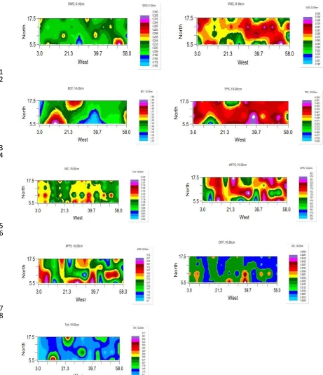
Interpolated maps portraying the distribution of soil properties across the field are shown in Fig. 9
2. Gravimetric water content (GWC) showed a good spatial distribution across the field with the 10
highest values located around the southwestern portion of the field. Volumetric water content 11
very pronounced, there were areas on the field that had slightly higher amount of these physical 16
properties than the rest of the field. In general, bulk density, total pore space, volumetric air 17
content, water filled pore space, air filled pore space, diffusivity, and tortuosity were very high in 18
the field even though they didn‟t exhibit very distinguishable variability. This lack of visible 19
13
Results of this study indicated that the spatial variability of soil water content (GWC and VWC) 1
was high. This can be explained by soil type (clay- loam) which was able to hold more water. But 2
with intensive tillage, this soil water content could be adversely affected. Studies have shown 3
that tillage practices can alter soil physical properties and consequently the hydrological behavior 4
of agricultural fields, especially when a similar tillage system has been practiced for a long 5
period [15, 28, 29, 30, 31]. Tillage intensity has also considerable effects on spatial structure and 6
spatial variability of soil properties [15, 30]. Therefore, this study can help determine site-7
specific soil management and decision making. To do so, spatial variability of the soil properties 8
properties on the field. Also, the sill (Co+C) can help determine where the variability or change 14
in soil property stops. This will be useful especially for irrigation purposes. 15
Generally, with farmers facing the decision of whether or not to till and the intensity of tillage, a 16
spatial variability study can help in this decision making. Maps produced in this study can also 17
be used for irrigation purposes as they can clearly indicate which portion of the field needs 18
irrigation (soil water content). Since different range of spatial dependence among soil properties 19
shows differences in response to human interferences and land use-cover, this will help reduce 20
human activities that increase soil bulk density and cause soil compaction like the use of heavy 21
equipments. It can also serve as a reference for the type of crop to be grown (cover crops for 22
14 1
2
4. Conclusion 3
We conducted a study in central Missouri to test the variability of soil physical properties in a 4
clay-loam soil. Results show variability in soil physical properties with depth and across the 5
field. Soil physical properties either decreased or increased sharply in the second depth (due to 6
the presence of a smectite layer) before leveling up or dropping off, but without reaching the first 7
depth value in either case. In addition, depending on soil physical property, maps produced by 8
krigging showed either good or poor spatial distribution. The semivariogram analysis showed 9
the presence of a strong (≤ 25%) to weak (>75%) spatial dependence of soil properties. Our 10
understanding of the behavior of soil properties in this study provides new insights for soil site-11
specific management in addressing issues such as „„where to place the proper interventions‟‟ 12
(tillage, irrigation and crop type to be grown). 13
14
15
Acknowledge ment 16
This research is part of a regional collaborative project supported by the USDA-NIFA, Award 17
No. 2011-68002-30190, “Cropping Systems Coordinated Agricultural Project: Climate Change, 18
Mitigation, and Adaptation in Corn-based Cropping Systems.” Project Web site: 19
http://sustainablecorn.org
20
21
22
15 References
1
[1] Schimel D, Melillo J, Tian H, McGuire D, Kicklighter D, Kittel T, Rosenbloom N, 2
Running S, Thornton P, Ojima D, Parton W, Kelly R, Sykes M, Neilson R, Rizzo B. 3
2000. Contribution of increasing CO2 and climate to carbon storage by ecosystems in the 4
United States. Science 287: 2004-2006. 5
[2] Kosmas C, Gerontidis S, Marathianou M. 200. The effects of land use change on soils and 6
vegetation over various lithological formations on Lesvos (Greece). Catena 40, 51-68. 7
[3] Igbal J. Thomasson JA, Jenkins JN, Owens PR, Whisler FD. 2005. Spatial variability analysis 8
of soil physical properties of alluvial soils. Soil Science Society of America Journal 69: 1-9
14. 10
[4] Zhang S, Zhang X, Huffman T, Liu X, Yang J. 2011. Influence of topography and land 11
management on soil nutrients variability in Northeast China. Nutrient Cycle & 12
Agroecosystem 89: 427-438. 13
[5] Munkholm, L.J., A. Garbout, S.B. Hansen. 2013. Tillage effects on topsoil structural quality 14
assessed using X-ray CT, soil cores and visual soil evaluation. Soil & Tillage Research 15
128, 104–109. 16
[6] Franzluebbers, A.J., 2002. Soil organic matter stratification ratio as an indicator of soil 17
quality. Soil and Tillage Research 66, 95–106. 18
[7] Munkholm, L.J., Schjønning, P., Rasmussen, K.J., Tanderup, K., 2003. Spatial and temporal 19
effects of direct drilling on soil structure in the seedling environment. Soil and Tillage 20
16
[8] Swarowsky, A., R.A. Dahlgren, K.W. Tate, J.W. Hopmans, A.T. O‟Geen.2011 Catchment-1
scale soil water dynamics in a Mediterranean-type oak woodland. Vadose Zone Journal, 2
10, 800-815. 3
[9] Webster R, Oliver MA. 1990. Statistical methods in soil and land Resource Survey. Oxford 4
University Press, Oxford University Press, Oxford, UK. 5
[10] Saldana A, Stein A, Zinck JA. 1998. Spatial variability of soil properties at different scales 6
within three terraces of the Henare River (Spain). Catena 33: 139-153. 7
[11] Wang ZM, Song KS, Zhang B, Liu DW, Li XY, Ren CY, Zhang SM, Lou L, Zhang CH. 8
2009. Spatial variability and affecting factors of soil nutrients in croplands of Northeast 9
China: a case study in Dehui county. P lant, Soil & Environment 55: 110-120. 10
[12] Webster R. 1985. Quantitative spatial analysis of soil in the field. In: Stewart, B.A. (Ed.), 11
Advances in Soil Science 3: 1-70. 12
[13] Pohlmann H. 1993. Geostatistical modeling of environmental data. Catena 20, 191-198. 13
[14] Cambardella CA, Moorman TB, Novak, JM, Parkin TB, Karlen DL, Turco RF, Konopka 14
AE. 1994. Field-scale variability of soil properties in central Iowa soils. Soil Science 15
Society of America Journal 58: 1501-1511. 16
[15] Ozgoz E. 2009. Long term conventional tillage effect on spatial variability of some soil 17
physical properties. Journal of Sustainable Agr iculture 33: 142-160. 18
[16] Nkongolo NV, Hatano R, and Kakembo V. 2010. Diffusivity models and greenhouse gases 19
fluxes from a forest, pasture, grassland and corn field in northern Hokkaido. Pedosphere 20
17
[17] Ayoubi SH, Zamani SM, Khomali F. 2007. Spatial variability of some soil properties for 1
site-specific farming in northern Iran. International Journa l of Plant Production 2: 225-2
236. 3
[18] Burgess TM, Webster R. 1980. Optimal Interpolation and isarithmic mapping of soil 4
properties: I. The variogram and punctual krigging. Journa l of Soil Science 31: 315-331. 5
[19] Parfitt JMB, Timm LC, Pauletto EA, Sousa RO, Castilhos DD, de Avila CL, Reckziegel 6
NL. 2009. Spatial variability of the chemical, physical and biological properties in 7
lowland cultivated with irrigated rice. Rev. Bra s. Cienc. Solo 33: 819-830. 8
[20] Grego CR, Vieira SR, Lourencao AL. 2006. Spatial distribution of Pseudaletia sequax 9
Franclemlont in triticale under no-till management. Science & Agr iculture 63: 321-327. 10
[21] Tesfahunegn GB, Tamane L, Vlek PLG. 2011. Catchment-scale spatial variability of soil 11
properties and implications on site-specific soil management in northern Ethiopia. Soil 12
& Tillage Research 117: 124-139. 13
[22] Grecu SJ, Kirkham MB, Kanemasu ET, Sweeney DW, Stone LR, Milliken GA. 1988. Root 14
growth in a claypan with a perennial-annual rotation. Soil Sci. Soc. Am. J. 52: 488-494 15
[23] Myers DB, Kitchen NR, Sudduth KA, Miles RJ, Sharp RE. 2007. Soybean root distribution 16
related to claypan soil properties and apparent soil electrical conductivity. Crop Sci. 47: 17
1498-1509 18
[24] Jiang P., Kitchen N.R., Anderson S.H., Sadler E.J., Sudduth K.A. 2008. Estimating palnt 19
available water using the simple inverse yield model for claypan landscapes. Agronomy 20
Journal. 100: 1-7. 21
[25] Utset A, Ruiz ME, Herrera J, Ponce de Leon D. 1998. A geostatistical method for soil 22
18
[26] Fu W, Tunney H, Zhang C. 2010. Spatial variation of soil nutrients in a dairy farm and its 1
implications for site-specific fertilizer application. Soil & Tillage Resea rch 106: 185-193. 2
[27] Lopez-Grandos F, Jurado-Exposito M, Atenciano S. Garcia-Ferrer A, De la Orden MS, 3
Garcia-Torres L. 2002. Spatial variability of Agricultural soil parameters in southern 4
Spain. Plant Soil 246: 97-105. 5
[28] Hill RL. 1990. Long-term conventional and no-tillage effects on selected soil physical 6
properties. Soil Science Society of America Journal 54: 161-166. 7
[29] Buschiazzo DE, Panigatti JL, Unger PW. 1998. Tillage effects on soil properties and crop 8
production in subhumid and semiarid Argentinean Pampas. Soil & Tillage Research 49: 9
105-116. 10
[30] Tsegaye T, Hill RL. 1998. Intensive tillage effects on spatial variab ility of soil physical 11
properties. Soil Science 163: 143-154. 12
[31] Gomez JA, Giraldez JV, Pastor M, Fereres E. 1999. Effects of tillage method on soil 13
physical properties, infiltration and yield in an olive orchard. Soil & Tillage Resea rch 52: 14
167-175. 15
16
17
18
19
19 1
Fig. 1. Study area (Lincoln University‟s Freeman farm) showing the plots 2
3
4
5
6
7
8
9
10
11
12
20 1
2
3 4
5
6
7
8
9
Fig. 2. Spatial distribution of soil physical properties at four depths in a clay-loam soil 10
21 1
a) Soil Bulk Density 2
3
22 1
c) Total Pore Space (TPS) 2
3
d) Volumetric Water Content (VWC) 4
5
Fig. 3a, b, c, d. Variation of soil physical properties with depth 6
23 1
Table 1. Descriptive statistics for soil physical properties at four depths in a clay- loam soil 2
AFPS: Air filled pore space (%); BDY: Soil bulk density (gcm-3); Diff.: Re lative gas diffusion coeffic ient (m2s-1m
-3
2
s); GWC: Gravimetric water content of soil (g.g-1); TPS: Total pore spaces (cm3cm-3); Tort.: Pore tortuosity factor
24 1
25
DSD = Degree of spatial dependence: strong DSD (DSD ≤ 25%), moderate DSD (25 < DSD ≤ 75%), 1
weak DSD (DSD > 75%) according to Cambardella et al., (1994). 2
3