Bioinformatics
Biocomputing and
Perl
An Introduction to Bioinformatics
Computing Skills and Practice
Michael Moorhouse
Post-Doctoral Worker from Erasmus MC,
The Netherlands
Bioinformatics
Biocomputing and
Perl
An Introduction to Bioinformatics
Computing Skills and Practice
Michael Moorhouse
Post-Doctoral Worker from Erasmus MC,
The Netherlands
West Sussex PO19 8SQ, England
Telephone (+44) 1243 779777
Email (for orders and customer service enquiries): [email protected] Visit our Home Page on www.wileyeurope.com or www.wiley.com
All Rights Reserved. No part of this publication may be reproduced, stored in a retrieval system or transmitted in any form or by any means, electronic, mechanical, photocopying, recording, scanning or otherwise, except under the terms of the Copyright, Designs and Patents Act 1988 or under the terms of a licence issued by the Copyright Licensing Agency Ltd, 90 Tottenham Court Road, London W1T 4LP, UK, without the permission in writing of the Publisher. Requests to the Publisher should be addressed to the Permissions Department, John Wiley & Sons Ltd, The Atrium, Southern Gate, Chichester, West Sussex PO19 8SQ, England, or emailed to [email protected], or faxed to (+44) 1243 770620.
This publication is designed to provide accurate and authoritative information in regard to the subject matter covered. It is sold on the understanding that the Publisher is not engaged in rendering professional services. If professional advice or other expert assistance is required, the services of a competent professional should be sought.
Other Wiley Editorial Offices
John Wiley & Sons Inc., 111 River Street, Hoboken, NJ 07030, USA
Jossey-Bass, 989 Market Street, San Francisco, CA 94103-1741, USA
Wiley-VCH Verlag GmbH, Boschstr. 12, D-69469 Weinheim, Germany
John Wiley & Sons Australia Ltd, 33 Park Road, Milton, Queensland 4064, Australia
John Wiley & Sons (Asia) Pte Ltd, 2 Clementi Loop #02-01, Jin Xing Distripark, Singapore 129809 John Wiley & Sons Canada Ltd, 22 Worcester Road, Etobicoke, Ontario, Canada M9W 1L1
Wiley also publishes its books in a variety of electronic formats. Some content that appears in print may not be available in electronic books.
British Library Cataloguing in Publication Data
A catalogue record for this book is available from the British Library
ISBN 0-470-85331-X
Typeset in 9.5/12.5pt Lucida Bright by Laserwords Private Limited, Chennai, India Printed and bound in Great Britain by Antony Rowe Ltd, Chippenham, Wiltshire
For my parents, who taught me the value of
knowledge – MJM
Contents
Preface xv
1 Setting the Biological Scene 1
1.1 Introducing Biological Sequence Analysis 1
1.2 Protein and Polypeptides 4
1.3 Generalised Models and their Use 5
1.4 The Central Dogma of Molecular Biology 6
1.4.1 Transcription 6
1.4.2 Translation 7
1.5 Genome Sequencing 10
1.5.1 Sequence assembly 11
1.6 The Example DNA-gene-protein system we will use 12
Where to from Here 13
2 Setting the Technological Scene 15
2.1 The Layers of Technology 15
2.1.1 From passive user to active developer 16
2.2 Findingperl 17
2.2.1 Checking forperl 17
Where to from Here 18
I
Working with Perl
19
3 The Basics 21
3.1 Let’s Get Started! 21
3.1.1 Running Perl programs 22
3.1.2 Syntax and semantics 23
3.1.3 Program: run thyself! 25
3.2 Iteration 26
3.2.1 Using the Perlwhileconstruct 26
3.3 More Iterations 30
3.3.1 Introducing variable containers 31
3.4 Selection 34
3.4.1 Using the Perlifconstruct 35
3.5 There Really is MTOWTDI 36
3.6 Processing Data Files 41
3.6.1 Askinggetlinesto do more 43
3.7 Introducing Patterns 44
Where to from Here 46
The Maxims Repeated 46
4 Places to Put Things 49
4.1 Beyond Scalars 49
4.2 Arrays: Associating Data with Numbers 49
4.2.1 Working with array elements 51
4.2.2 How big is the array? 51
4.2.3 Adding elements to an array 52
4.2.4 Removing elements from an array 54
4.2.5 Slicing arrays 54
4.2.6 Pushing, popping, shifting and unshifting 56 4.2.7 Processing every element in an array 57
4.2.8 Making lists easier to work with 59
4.3 Hashes: Associating Data with Words 60
4.3.1 Working with hash entries 61
4.3.2 How big is the hash? 61
4.3.3 Adding entries to a hash 62
4.3.4 Removing entries from a hash 62
4.3.5 Slicing hashes 63
4.3.6 Working with hash entries: a complete example 64
4.3.7 Processing every entry in a hash 66
Where to from Here 68
The Maxims Repeated 68
5 Getting Organised 71
5.1 Named Blocks 71
5.2 Introducing Subroutines 73
5.2.1 Calling subroutines 73
5.3 Creating Subroutines 74
5.3.1 Processing parameters 76
5.3.2 Better processing of parameters 78
5.3.3 Even better processing of parameters 80
5.3.4 A more flexibledrawlinesubroutine 83
5.3.5 Returning results 84
5.4 Visibility and Scope 85
5.4.1 Using private variables 86
5.4.2 Using global variables properly 88
5.4.3 The final version ofdrawline 89
5.5 In-built Subroutines 90
5.6 Grouping and Reusing Subroutines 92
5.6.1 Modules 93
5.7 The Standard Modules 96
5.8 CPAN: The Module Repository 96
5.8.1 Searching CPAN 97
Contents ix
5.8.3 Installing a CPAN module automatically 99
5.8.4 A final word on CPAN modules 99
Where to from Here 100
The Maxims Repeated 100
6 About Files 103
6.1 I/O: Input and Output 103
6.1.1 The standard streams:STDIN,STDOUTandSTDERR 103
6.2 Reading Files 105
6.2.1 Determining the disk-file names 106
6.2.2 Opening the named disk-files 108
6.2.3 Reading a line from each of the disk-files 110
6.2.4 Putting it all together 110
6.2.5 Slurping 114
6.3 Writing Files 116
6.3.1 Redirecting output 117
6.3.2 Variable interpolation 117
6.4 Chopping and Chomping 118
Where to from Here 119
The Maxims Repeated 119
7 Patterns, Patterns and More Patterns 121
7.1 Pattern Basics 121
7.1.1 What is a regular expression? 122
7.1.2 What makes regular expressions so special? 122
7.2 Introducing the Pattern Metacharacters 124
7.2.1 The+repetition metacharacter 124
7.2.2 The|alternation metacharacter 126
7.2.3 Metacharacter shorthand and character classes 127
7.2.4 More metacharacter shorthand 128
7.2.5 More repetition 130
7.2.6 The?and*optional metacharacters 130
7.2.7 The any character metacharacter 131
7.3 Anchors 132
7.3.1 The\bword boundary metacharacter 132
7.3.2 The^start-of-line metacharacter 133
7.3.3 The$end-of-line metacharacter 133
7.4 The Binding Operators 134
7.5 Remembering What Was Matched 135
7.6 Greedy by Default 137
7.7 Alternative Pattern Delimiters 138
7.8 Another Useful Utility 139
7.9 Substitutions: Search and Replace 140
7.9.1 Substituting for whitespace 141
7.10 Finding a Sequence 142
Where to from Here 146
The Maxims Repeated 146
8 Perl Grabbag 147
8.1 Introduction 147
8.3 Perl One-liners 149
8.4 Running Other Programs fromperl 152
8.5 Recovering from Errors 153
8.6 Sorting 155
8.7 HERE Documents 159
Where to from Here 160
The Maxims Repeated 161
II
Working with Data
163
9 Downloading Datasets 165
9.1 Let’s Get Data 165
9.2 Downloading from the Web 165
9.2.1 Usingwgetto download PDB data-files 167
9.2.2 Mirroring a dataset 168
9.2.3 Smarter mirroring 168
9.2.4 Downloading a subset of a dataset 169
Where to from Here 171
The Maxims Repeated 171
10 The Protein Databank 173
10.1 Introduction 173
10.2 Determining Biomolecule Structures 174
10.2.1 X-Ray Crystallography 174
10.2.2 Nuclear magnetic resonance 176
10.2.3 Summary of protein structure methods 177
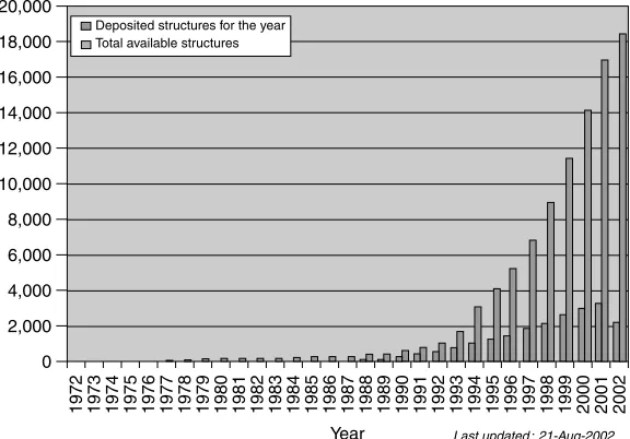
10.3 The Protein Databank 177
10.4 The PDB Data-file Formats 179
10.4.1 Example structures 180
10.4.2 Downloading PDB data-files 181
10.5 Accessing Data in PDB Entries 182
10.6 Accessing PDB Annotation Data 183
10.6.1 Free R and resolution 184
10.6.2 Database cross references 186
10.6.3 Coordinates section 188
10.6.4 Extracting 3D coordinate data 191
10.7 Contact Maps 192
10.8 STRIDE: Secondary Structure Assignment 196
10.8.1 Installation of STRIDE 197
10.9 Assigning Secondary Structures 197
10.9.1 Using STRIDE and parsing the output 200 10.9.2 Extracting amino acid sequences using STRIDE 204
10.10 Introducing themmCIFProtein Format 205
10.10.1 ConvertingmmCIFto PDB 206
10.10.2 ConvertingmmCIFsto PDB withCIFTr 206 10.10.3 Problems with theCIFTrconversion 208
10.10.4 Some advice on usingmmCIF 208
10.10.5 Automated conversion ofmmCIFto PDB 208
Where to from Here 210
Contents xi
11 Non-redundant Datasets 211
11.1 Introducing Non-redundant Datasets 211
11.1.1 Reasons for redundancy 211
11.1.2 Reduction of redundancy 212
11.1.3 Non-redundancy and non-representative 212
11.2 Non-redundant Protein Structures 213
Where to from Here 217
The Maxims Repeated 217
12 Databases 219
12.1 Introducing Databases 219
12.1.1 Relating tables 220
12.1.2 The problem with single-table databases 222
12.1.3 Solving the one-table problem 222
12.1.4 Database system: a definition 224
12.2 Available Database Systems 224
12.2.1 Personal database systems 225
12.2.2 Enterprise database systems 225
12.2.3 Open source database systems 225
12.3 SQL: the Language of Databases 226
12.3.1 Defining data with SQL 226
12.3.2 Manipulating data with SQL 227
12.4 A Database Case Study: MER 227
12.4.1 The requirement for the MER database 231
12.4.2 Installing a database system 232
12.4.3 Creating the MER database 233
12.4.4 Adding tables to the MER database 235
12.4.5 Preparing SWISS-PROT data for importation 238 12.4.6 Importing tab-delimited data intoproteins 245
12.4.7 Working with the data inproteins 246
12.4.8 Adding another table to the MER database 248 12.4.9 Preparing EMBL data for importation 249 12.4.10 Importing tab-delimited data intodnas 253
12.4.11 Working with the data indnas 253
12.4.12 Relating data in one table to that in another 254 12.4.13 Adding thecrossrefstable to the MER database 255 12.4.14 Preparing cross references for importation 256 12.4.15 Importing tab-delimited data intocrossrefs 259 12.4.16 Working with the data incrossrefs 259 12.4.17 Adding thecitationstable to the MER database 263 12.4.18 Preparing citation information for importation 265 12.4.19 Importing tab-delimited data intocitations 268 12.4.20 Working with the data incitations 268
Where to from Here 269
The Maxims Repeated 269
13 Databases and Perl 273
13.1 Why Program Databases? 273
13.2 Perl Database Technologies 274
13.3 Preparing Perl 275
13.4 Programming Databases withDBI 276 13.4.1 Developing a database utility module 279
13.4.2 Improving upondump results 280
13.5 Customising Output 282
13.6 Customising Input 285
13.7 Extending SQL 289
Where to from Here 292
The Maxims Repeated 292
III
Working with the Web
295
14 The Sequence Retrieval System 297
14.1 An Example of What’s Possible 297
14.2 Why SRS? 298
14.3 Using SRS 298
Where to from Here 300
The Maxims Repeated 300
15 Web Technologies 303
15.1 The Web Development Infrastructure 303
15.2 Creating Content for the WWW 305
15.2.1 The static creation of WWW content 308 15.2.2 The dynamic creation of WWW content 308
15.3 Preparing Apache for Perl 310
15.3.1 Testing the execution of server-side programs 312
15.4 Sending Data to a Web Server 315
15.5 Web Databases 320
Where to from Here 327
The Maxims Repeated 327
16 Web Automation 329
16.1 Why Automate Surfing? 329
16.2 Automated Surfing with Perl 330
Where to from Here 335
The Maxims Repeated 336
IV
Working with Applications
337
17 Tools and Datasets 339
17.1 Introduction 339
17.2 Sequence Databases 340
17.2.1 Understanding EMBL entries 343
17.2.2 Understanding SWISS-PROT entries 346
17.2.3 Summarising sequences databases 347
17.3 General Concepts and Methods 347
17.3.1 Predictions and validation 348
Contents xiii
17.3.3 Balancing the errors 351
17.3.4 Using multiple algorithms to improve performance 352
17.3.5 tRNA-ScanSE, a case study 353
17.4 Introducing Bioinformatics Tools 357
17.4.1 ClustalW 358
17.4.2 Algorithms and methods 359
17.4.3 Installation and use 360
17.4.4 Substitution/scoring matrices 361
17.5 BLAST 362
17.5.1 Installing NCBI-BLAST 364
17.5.2 Preparation of database files for faster searching 365 17.5.3 The different types of BLAST search 369
17.5.4 Final words on BLAST 371
Where to from Here 371
The Maxims Repeated 371
18 Applications 373
18.1 Introduction 373
18.2 Scientific Background to Mer Operon 374
18.2.1 Function 374
18.2.2 Genetic structure and regulation 374
18.2.3 Mobility of the Mer Operon 375
18.3 Downloading the Raw DNA Sequence 377
18.4 Initial BLAST Sequence Similarity Search 378
18.5 GeneMark 380
18.5.1 Using BLAST to identify specific sequences 382 18.5.2 Dealing with false negatives and missing proteins 386 18.5.3 Over-predicted genes and false positives 387 18.5.4 Summary of validation of GeneMark prediction 388
18.6 Structural Prediction with SWISS-MODEL 388
18.6.1 Alternatives to homology modelling 390
18.6.2 Modelling with SWISS-MODEL 390
18.7 DeepView as a Structural Alignment Tool 396
18.8 PROSITE and Sequence Motifs 401
18.8.1 Using PROSITE patterns and matrices 402 18.8.2 Downloading PROSITE and its search tools 403
18.8.3 Final word on PROSITE 407
18.9 Phylogenetics 407
18.9.1 A look at the HMA domain ofMerAandMerP 407
Where to from Here? 410
The Maxims Repeated 411
19 Data Visualisation 413
19.1 Introducing Visualisation 413
19.2 Displaying Tabular Data Using HTML 415
19.2.1 Displaying SWISS-PROT identifiers 417
19.3 Creating High-quality Graphics with GD 422
19.3.1 Using theGDmodule 424
19.3.2 Displaying genes in EMBL entries 426
19.4 Plotting Graphs 431 19.4.1 Graph-plotting using theGD::Graphmodules 432
19.4.2 Graph-plotting using Grace 433
Where to from Here 439
The Maxims Repeated 439
20 Introducing Bioperl 441
20.1 What is Bioperl? 441
20.2 Bioperl’s Relationship to Project Ensembl 442
20.3 Installing Bioperl 442
20.4 Using Bioperl: Fetching Sequences 444
20.4.1 Fetching multiple sequences 445
20.4.2 Extracting sub-sequences 447
20.5 Remote BLAST Searches 448
20.5.1 A quick aside: theblastcl3 NetBlastclient 449
20.5.2 Parsing BLAST outputs 450
Where to from Here 451
The Maxims Repeated 452
A Appendix A 453
B Appendix B 457
C Appendix C 459
D Appendix D 461
E Appendix E 467
F Appendix F 471
Preface
Welcome toBioinformatics, Biocomputing and Perl, an introduction and guide to the computing skills and practices collectively known asBioinformatics.
Bioinformatics is the application of computing techniques to the study of biology, and in particular biology research. Although the study of biology is hundreds of years old, the application of computing techniques to biology research is relatively new, with major advances occurring within the last decade. Consequently, the Bioinformatics field is evolving and maturing rapidly, and this has highlighted the need for a good, all-round introductory textbook. We believe thatBioinformatics, Biocomputing and Perlmeets this need.
What is in this Book?
After two introductory chapters,Bioinformatics, Biocomputing and Perlis divided into four main parts:
1. Working with Perl. 2. Working with Data. 3. Working with the Web. 4. Working with Applications.
Part I, Working with Perl, introduces programming to the student of Bioinfor-matics. Note that the intention is not to turn Bioinformaticians into software engineers. Rather, the emphasis is on providing Bioinformaticians with program-ming skills sufficient to enable them to produce bespoke programs when required in the course of their research.
scripting capabilities. If that sounds liketechno babble, do not worry; the impor-tance of these programming language features is explained in a less technical way later. Fortunately, Perl is not particularly difficult to learn. For instance, by the end of Chapter 3, the reader will know enough Perl to be able to produce simple, but useful, programs. This early material is then developed so that by the end of Part I, readers will be able to confidently create customised and customisable programs to solve diverse Bioinformatics problems.
In Part II, Working with Data, the emphasis shifts from creating bespoke Bioinformatics programs to exploring the tools and techniques used to organise, store, retrieve and process data. After explaining how to download datasets from the Internet, the Protein DataBank (PDB) is described in detail. A short chapter follows on the importance of non-redundant datasets, before discussion shifts to cover relational database management systems. How to create and use databases with the popularMySQLtool is described. In addition to using standard tools to interact with databases, the use of Perl programs to interrogate databases is also covered.
Part III, Working with the Web, covers a collection of web-based technologies that, once mastered, can be used to publish research -- both findingsanddata -- on the Internet. Electronic mechanisms allowing interaction with, and interrogation of, web-based data are explained. Perl again plays an important role in this part of the book, with HTML and CGI also covered.
Part IV,Working with Applications, describes a set of standard Bioinformatics tools and applications. Although it is often useful to be able to create a new tool from scratch, it can sometimes be more appropriate to take existing tools and control their execution and interaction. Scripting technologies, of which Perl is only one type, are particularly useful in this area. A discussion of ‘‘The Bioperl Project’’, and its importance, completesBioinformatics, Biocomputing and Perl.
Maxims, Commentaries, Exercises and Appendices
All but the first two chapters contain a collection of maxims. These are your authors’snippets of wisdom. At the end of each chapter, the maxims are repeated in list form. If, having worked through a chapter, the maxims are understood, it is an indication that the associated material has been understood. If, however, a maxim is not understood, it indicates that there is a need to review the material to which the particular maxim relates.
In addition to the maxims, chapters include technical commentaries. Unlike maxims, it is not necessary to fully understand the commentaries on first reading. If a technical commentary is not immediately understood, it is possible to safely continue to work through the text without too much difficulty.
Preface xvii
exercises are worked through, as it is only through practice and review that Bioinformatics computing skills are developed and honed.
A collection of appendices completes the book, providing information on, among other things, installing Perl on various platforms, the Perl on-line doc-umentation and a list of Perl operators. An annotated list of references and suggestions for further reading are also presented as an appendix.
Who Should Read this Book
This book targets three distinct readerships.
The main target is the student of biology, both under- and post-graduate. Bioin-formatics, Biocomputing and Perl is designed to be themust-have, introductory Bioinformatics textbook. The biology student taking a Bioinformatics module will find this book to be a useful starting point and an essential desktop reference.
Another target is the qualified, professional or academic biologist who needs to understand more about Bioinformatics. The field of Bioinformatics is still relatively new and it is only now appearing as a feature within biology course outlines and syllabi. However, there are many qualified biologists ‘‘in the field’’ requiring a good primer. This book is designed to meet that need.
The final target is the computer scientist curious to understand how computing skills might be used within this growing field.
What you Should know Already
It is assumed that some knowledge of computer use has already been acquired, including understanding the concept of a disk-file and knowing how to create one using an editor. On the Linux operating system, popular editors arevi,picoand emacs. On any of the Windows operating systems, Notepad,WordPadandWord are all editors, although the latter is a more sophisticated example. Macintosh users haveSimpleTextandBBedit. Any of these will suffice, so long as it allows for the creation and manipulation of plain text files. Later chapters (Parts III and IV) assume a working knowledge of HTML.
Platform Notes
system. Two additional appendices provide a list of essential Linux commands and a quick reference to thevitext editor, respectively.
Accompanying Web-site
Details of the book’s mailing list, its source code, any errata and other related material can be found on the book’s web-site, located at:
http://glasnost.itcarlow.ie/~biobook/index.html
Your Comments are Welcome
The authors welcome all comments aboutBioinformatics, Biocomputing and Perl. Send an e-mail to either of the following addresses:
Acknowledgements
Michael thanks his parents for their unwavering support, be it material, practical or emotional. Their endless hours of reading and re-reading the draft chapters and manuscript produced many points of very welcome constructive criticism. Although completing a PhD., moving country and starting a new job while writing a book is not something he’d recommend, Michael thanks those around him for helping when they could and for understanding why he was so busy. Also, thanks to all in the new Department of Bioinformatics, Erasmus MC, the Netherlands, who have offered their support and understanding.
Preface xix
months late! This book’s editorial assistant was Layla Paggetti, and both authors thank Layla for her prompt and efficient responses to their many queries. Robert Hambrook acted as production editor. As with Paul’s first book, this one has benefited greatly from Robert’s management of the production process.
1
Setting the
Biological Scene
Introducing DNA, RNA, polypeptides, proteins and sequence
analysis.
1.1
Introducing Biological Sequence Analysis
Among other things, this book describes a number of techniques used to analyse DNA, RNA and proteins.
To a molecular biologist, DNA is a very physical molecule: a polymer of nucleotides that are collectively calleddeoxyribose nucleic acid. It coils, bends, flexes and interacts with proteins, and is generally interesting. RNA is similar to DNA in structure, but for the fact that RNA contains the sugarriboseas opposed todeoxyribose. DNA has a hydrogen at the second carbon atom on the ring; RNA has a hydrogen linked through an oxygen atom.
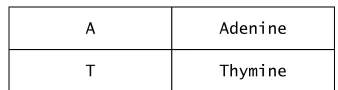
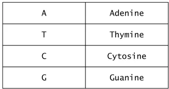
In DNA and RNA, there are four nucleotide bases. Three of these bases are the same: guanine (G), adenine (A) and cytosine (C). The fourth base for DNA is thymine (T), whereas in RNA, the fourth base lacks a methyl group
and is called uracil (U). Each base has two points at which it can join cova-lently to two other bases on either end, forming a linear chain of monomers. These chains can be quite long, with many millions of bases common in most organisms.
Bioinformatics, Biocomputing and Perl. Michael Moorhouse and Paul Barry c
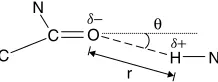
Figure 1.1 Adenine (A) and thymine (T) nucleotide bases (where the thin black lines indicate the three hydrogen bonds between the two bases).
Another interesting feature of nucleotide bases is that the four bases hydrogen-bondtogether in two exclusive pairs because of the position of the charged atoms along their edges, as shown in Figure 1.1 on page 2 and Figure 1.2 on page 31. Three of these bonds form between C and G, whereas two form between A and T (or A and U in RNA).
These bonds, while considerably weaker than the covalent bonds between atoms, are enough to stabilise structures such as the famous double helix, in which the bases line up nearly perpendicular to the axis of the helix, as shown in Figure 1.3 on page 4. There are several important consequences of thedouble helix:
• Where there is a G in one chain, there is a C in the corresponding location in the other, and the two chains are said to becomplementary to each other. The chains are often referred to asstrands.
• This complementarity means that there is 50% redundancy in the informa-tion stored in both chains; consequently, only one chain is needed to store all the information for both (as one can be deduced from the other)2.
• Because of the structure of the nucleotide bases, DNA molecules have
direction. This is a subtle, but important, point. The phosphate backbones
attachto the sugar rings at different locations: the 3’ and 5’ hydroxyl groups.
1
These diagrams were produced withOpen Rasmolon the basis of protein structure1D66.
2
Introducing Biological Sequence Analysis 3
Figure 1.2 Guanine (G) and cytosine (C) nucleotide bases (where the thin black lines indicate the three hydrogen bonds between the two bases).
When DNA is run in opposite directions, one end of the helix is the 3’ end of one chain and the 5’ end of the other. When the order of the nucleotide bases is written down, it is conventional to start at the nucleotides at the 5’ (the ‘left-most’ nucleotide) end of the DNA molecule and work towards the 3’ end at the right (the ‘right-most’ base). The importance of this directional feature will become clear later in this chapter, when open reading frames
are described.
In general, RNA copies of DNA are made by a process known as transcription. For most purposes, RNA can be regarded as aworking copy of the DNAmaster template. There is usually one or a very small number of examples of DNA in the cell, whereas there are multiple copies of the transcribed RNA.
A common term related to the number of nucleotide bases in a particular sequence is a reference tobase pairs3, for example ‘‘400 base pairs’’. This term is a generic term that can literally mean ‘‘400 paired bases’’. More often, though, it is used to acknowledge that while there are 400 nucleotides in a particular sequence being actively considered, there are another 400 nucleotides on the complementary strand running in the other direction. In this context, the use of base pairs is a tacit acknowledgement of their existence that may be of great importance, as the feature under investigation may be on the other strand. In nearly all cases, both strands should be considered.
There are many interesting features of DNA. As this discussion is an overview, a description of some of these features (such aspromoters,splice sites,intron/exon boundariesandgenes) is deferred until later chapters.
3
Figure 1.3 The DNA ‘‘double helix’’ (where the backbones, in black, run in opposite directions).
1.2
Protein and Polypeptides
DNA is thenobilityof the cellular world. Proteins are theworker-serfs.
To a biochemist, proteins are the functioning units of cellular life. Proteins do physically useful things such as catalysing reactions, processing energy rich molecules, pumping other molecules across cellular barriers and forming con-nective and motility structures. Proteins do just about anything else in the cell that can be considered ‘‘real work’’.
In molecular terms, proteins are chains technically termed polypeptides and formed from 20 different types ofamino acids. These may be modified in different ways to alter their properties, the structure that is formed and the final function of the molecule. For example, certain amino acids can beglycosylated4, which can be used as recognitiontags, while other proteins associate with small molecules calledligandsthat have special properties useful in the catalysis of reactions.
The structure of a protein is generally more variable than DNA. It is at the level of proteins that the variety of the information contained in the order of DNA bases is used. The result is that the amino acid chain producedfoldinto structures that are closely linked to that particular protein’s functional role within the cell (and these can vary enormously). This folding has another important consequence in that parts of a protein (i.e. its amino acids) can be physically close together in space, but distant in terms of their location in the sequence of the amino acids.
Consider, as an example, the well-studiedcatalytic triad of chymotrypsin. The critical parts of the protein for its function (which is to degrade other proteins) are the amino acidsasparateat position 102 in the polypeptide chain,histidine
at 57 andserineat 195. The triad is presented in Figure 1.4 on page 5. The right-hand side of the image shows the catalytic site in close-up, with the three critical amino acids located closely in physical space, but distant in sequence. The inset (left-hand image) shows the general structure of the protein demonstrating how the complex folding of the chain brings these residues together.
4
Generalised Models and their Use 5
Histidine 57
Serine 195
Asparate 102
Figure 1.4 The catalytic triad of chymotrypsin (PDB ID: 1AFQ).
1.3
Generalised Models and their Use
The relationships between DNA, RNA, protein, structure and function follow a generalised model. Unfortunately, like most generalisations, it is oversimplistic for many situations. If this is the case, why use it? There are two good reasons:
1. The model is a ‘‘good enough’’ description of what happensmost of the time. Certainly, there are important exceptions. There are non-standard amino acids included in proteins via some other mechanism (which are ignored in this book). Possibilities such as the section of DNA coding for single protein being discontinuous are additional complexities that are considered later. However, overall, the model is a valuable approximation to reality that has useful predictive power when working with new systems.
2. The model is a ‘‘lie-to-children’’5: it allows the basic features to be under-stood without confusing things by considering exceptions and enhance-ments. Once such a simple system is understood, it can be extended to cover more complex aspects and specific examples. In short, a start has to be made somewhere, and the generalised model is as good a place to start as anywhere.
Before considering the mechanisms by which information is conserved and convertedalong the pathway, let’s consider another important point about the abstract nature of the data to be used.
Bioinformaticians are generally concerned with information at an abstract level: DNA, RNA and amino acid sequences are ‘‘just’’ strings of letters. It is sometimes easy to forget that these are actual representations of molecules that exist in the cellular world and, consequently, must interact with the physical
5
universein general, let alone existing within a cellular environment. How much a Bioinformatician needs to know about the real-world context of the data being analysed depends on the analysis that is performed6. In some cases, quite superficial knowledge suffices, while others require a deeper understanding of the fundamental physical and biological processes at work.
Only through experience can the Bioinformatician hone the skill and profes-sional judgement necessary to decide how much understanding of the underlying biological system is needed for any particular analysis. The idealistic response is ‘‘the more the better’’, which is like all ideals: something to aim at but rarely achieved in practice. Time is often a factor for the Bioinformatician. If too long is spent becoming versed in the biological background, the risk of not completing an analysis within a useful timescale will increase. Conversely, there is also the risk of an analysis being compromised because too little is known about the system under study. This is where the balance between the two extremes comes in. This book attempts to guide the reader in this regard through the examples presented and provide useful pointers beyond. However, in the end, it all comes down toexperienceandprofessional judgement.
1.4
The Central Dogma of Molecular Biology
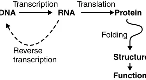
The DNA to Functional Protein Structure Model discussed above is often referred to as the ‘‘Central Dogma of Molecular Biology’’. It is summarised in a slightly extended form in Figure 1.5 on page 6. The arrows represent information flow
from that stored in the order of the DNA bases through the folding of the polypeptide chain to a fully functional protein.
1.4.1
Transcription
Transcriptionis the conversion of information from DNA to RNA, and is straight-forward because of the direct correspondence between the four nucleotide bases of DNA and those of RNA.
Transcription Translation
Reverse transcription
Folding
Structure
Function Protein RNA
DNA
Figure 1.5 The central dogma of molecular biology.
6
The Central Dogma of Molecular Biology 7
There is an interesting exception inRNA Retroviruses, the most famous example being HIV (the Human Immunodeficiency Virus) that causes AIDS. In retroviruses, RNA is used as the information storage material. This is then copied (badly in the case of HIV) into DNA, which then integrates into the nucleic acid material of the cell under attack. This ‘‘trick’’ allows the virus (and its information) to lie dormant for long periodsin relative safety, whereas the original RNA material is more likely to be actively degraded by cellular enzymes.
This RNA to DNA conversion ability is also useful for molecular biologists, as DNA can be more easily stored or manipulated using standard techniques. This has important implications, which are discussed later.
1.4.2
Translation
In a protein-coding region of DNA, three successive nucleotide bases, called
tripletsor codons, are used to code for each individual amino acid. Three bases are needed because there are 20 amino acids but only four nucleotide bases: with one base there are four possible combinations; with two bases, 16 (42); with three, 64 (43), which is more than the number of amino acids.
TheRNA transcriptis used by a complex molecular machine called theribosome
to translate the order of successive codons into the corresponding order of amino acids. Specialstop codons, such as UAA, UAG and UGA, induce the ribosometo terminate the elongation of the polypeptide chain at a particular point. Similarly, the codon for the amino acidmethionine(AUG in RNA) is often used as thestart signalfor translation.
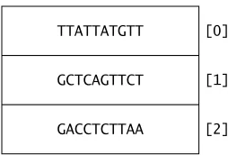
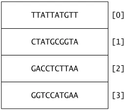
The section of DNA between the start and stop codons is called an open reading frame. There is a complication in that the codons found depend on how the sequence of nucleotide bases is divided. This is dependent on where the count starts. There is no biological reason why the first nucleotide base reported in a DNA sequence should be related to the protein coding regions.
A common solution is to calculate the codons produced from all possible open reading frames and select the most plausible on the basis of the results. The
correctopen reading frame for a particular region of DNA is generally that which has the longest distance between any start and stop codons. Though there are exceptions, especially in some viruses and bacteria, each nucleotide is involved in coding for only one amino acid and, hence, only one open reading frame is correct. The incorrect reading frames are generally short and as a consequence, do not resemble recognisable proteins.
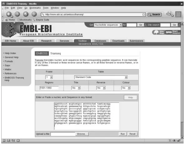
Figure 1.6 The EMBOSS/Transeq page at the EBI.
the sequence under study are referred to as +1, +2 and +3, while those on the complement strand are−1,−2 and−3.
The effects of choosing the correct and incorrect reading frames can be investigated using theTranseqtool contained in theEMBOSSsuite of programs. As these tools are discussed later in this book, a number of the details are glossed over here in favour of illustrating the point at hand. Figure 1.6 on page 8 shows theTranseqinterface provided by the EBI at the following Internet address:
http://www.ebi.ac.uk/emboss/transeq/
For this example, consider bases Bases 1501 through 1800 from EMBL entry
M245940. This sequence is chosen because it contains the MerP protein. These particular bases are easy to extract from a disk-file using any text editor. From the entry, the six lines of DNA bases (near the end of the EMBL data-file) can be copied. The line numbers at the end of each line can be removed and then the resulting data can be pasted into the box on EMBOSS/Transeq WWW form (refer to Figure 1.6). Here’s what the data looks like before the editing takes place:
The Central Dogma of Molecular Biology 9
acgctgtccg taccgggcat gacctgctcc gcttgtccga tcaccgttaa gaaggcgatt 1680 tccaaggtcg aaggcgtcag caaagttaac gtgaccttcg agacacgcga agcggttgtc 1740 accttcgatg atgccaagac cagcgtgcag aagctgacca aggccaccga agacgcgggc 1800 tatccgtcca gcgtcaagaa gtgaggcact gaaaacggca gcgcagcaca tctgacgccc 1860
If desired, the space between each group of ten letters can be removed using any editor’s search-and-replacefunction. However, in the raw sequence, space characters and newlines are ignored, so it is OK to leave them as-is when pasting the data into the form.
The stand-alone, command-line version of Transeq has a parameter, called
-regions, that restricts translation to a specified range of bases. To use this feature on the WWW form, insert ‘‘1501-1860’’ into the ‘‘Regions’’ box.
Technical Commentary: Note that the line numbers on the right-hand side of the above extracted data are actually the index of the last base on the line. This means that 1501 is the first base on the line that ends with 1560, as the bases are arranged in six blocks of ten per line.
The results of this web-run are not shown. Here is the correct result, which is reading frame +1 relative to the start point of the sequence just selected:
GFPYVMPFFY*SQEFIMKKLFASLAIAAVVAPVWAATQTVTLSVPGMTCSACPITVKKAI SKVEGVSKVNVTFETREAVVTFDDAKTSVQKLTKATEDAGYPSSVKK*GTENGSAAHLTP
The underlined section is the MerP protein sequence. It starts with a Methionine (M)startsignal codon, which is ATG, as this is the DNA representation, not RNA. It ends with * stop codon (which is TGA in DNA). The start and stop codons are underlined in the original sequence block above. The rest of the triplet of bases (the other codons) are translated by looking them up in standard codon translation tables. These vary very little between organisms.
This translation of the DNA for the MerP protein is also documented in the EMBL disk-file in annotation included with the originalM15049 EMBL entry’sFT
annotation (where ‘‘F’’ and ‘‘T’’ are taken from ‘‘feature’’):
FT CDS 1549..1824
FT /codon_start=1
FT /db_xref="GOA:P13113" FT /db_xref="SWISS-PROT:P13113" FT /transl_table=11
FT /gene="merP"
FT /product="mercury resistance protein" FT /protein_id="AAA98223.1"
FT /translation="MKKLFASLAIAAVVAPVWAATQTVTLSVPGMTCSACPITVKKAIS FT KVEGVSKVNVTFETREAVVTFDDAKTSVQKLTKATEDAGYPSSVKK"
Note that all of the hard work is already done, including a cross reference to the SWISS-PROT database (the ‘‘/db xref=SWISS-PROT:P13113’’ bit) as well as the official translation of the DNA sequence7.
7
This introduction is purposefully straightforward. Things become more dif-ficult when all that’s at hand is a small piece of DNA, the order of the bases and, maybe, the name of the organism. Using these data to identify a protein is returned to later inBioinformatics, Biocomputing and Perl.
Once produced, the polypeptide chain must by folded in order to become an active protein in the functional form. A common assertion is that all the information needed to produce the defined structure of the fully functional protein is contained in the amino acid sequence. In a very general sense, this is true. However, it is only correct when the environment within which the polypeptide exists is taken into account.
1.5
Genome Sequencing
The sequencing of an entire genome – the DNA content of a particular organ-ism – is now relatively routine. Originally, it was performed in a very ‘‘cottage industry’’ way, with small groups of researchers working away, in relative isola-tion, at sequencing small sections of the complete genome.
Today, genome sequencing is ‘‘big science’’, and there are numerous specialised genome sequencing centres around the world, such as The WelcomeTrust Sanger Institute in the United Kingdom and The Center for Genome Research in the United States. A number of commercial organisations sequence genomes on a for-profit basis, withCelera Genomicsthe most famous – some would say ‘‘infa-mous’’ – because of the company’s efforts to beat the publicly funded Human Genome Projectin being first to publish the draft human genome sequence. This was in an effort to copyright and/or patent the information and, consequently, charge money for the usage rights8.
In Bioinformatics, Biocomputing and Perl, the emphasis is on analysing the DNA and protein sequences rather than understanding the technical details of the methods by which the sequences are produced. However, it is important to have (at least) a rudimentary knowledge of the technologies used to produce the sequences. This allows the reader to better understand both the successes and the problems associated with the processes, as well as how they influence the data analysed. This description is very brief and intended to summarise the more thorough treatments found in any general biochemistry or molecular biology textbook.
Nowadays, most DNA is sequenced using theDideoxynucleotide (Chain Termi-nation) Method developed by Fredrick Sanger and his colleagues. This method uses a modifiedDNA polymerase enzymeto make copies of the DNA present in an original sample. As well as the normal DNA nucleotide bases present in the reaction mixture, specialdi-deoxy versionsare also included. These have hydro-gen atoms instead of hydroxyl groups in the ribose sugar at two positions: the
8
Genome Sequencing 11
2’ (as per normal DNA bases) and also at the 3’ position. This means that when the DNA polymerase adds a di-deoxy base to the elongating DNA chain, no more bases can be added to that chain. This is because the hydrogen at the 3’ position is non-reactive compared to the hydroxyl group normally present. The result is that the chain is essentiallyblocked from further extension at this length. As all four di-deoxy nucleotides are added to the reaction mixture, there will beblocked
examples of the DNA molecules that terminate at every base.
These molecules can be separated from each other by the use of a polyacry-lamide gel lattice, as shorter DNA molecules pass through it quickly, while longer ones take more time. Each di-dedoxy nucleotide is labelled with a different flu-orescent marker corresponding to the base type: A, T, G and C. This tag can be excited by a laser scanning at a particular location and the base passing that point at a particular time can beread off. The length of this ‘‘read’’ is typically about 500 bases before the separation between the molecules becomes too poor to deter-mine which molecule is passing under the laser excitation position. Actually, longer reads are possible but can result in reduced accuracy if special techniques are not employed. For the purposes of this book, 500 bases is assumed to be enough. Even if this were 250 or 1000, it would not algorithmically affect the next step, which is sequence assembly. All that’s required is to do more or less depending on the actual value chosen.
1.5.1
Sequence assembly
500 bp (base pairs nucleotides) is a short piece of DNA compared to the total found in organisms. This can code for a protein of slightly over 165 aminos9, which is a ‘‘none-too-large protein’’. Yet even viruses that are not self sufficient have many kilobases of DNA that have been sequenced. The general technique is to sequence many 500 bp regions and then stitch them back together. This has allowed the DNA sequence for a particular organism, commonly referred to as ‘‘The Genome’’, to be found. Nowadays, sequencing the genome is one of the standard stages in the analysis of any sufficiently interesting organism, and the
threshold of interest that must be reached before resources are committed to such a project continues to fall. The process is as follows:
• An individual organism (or a range of individual organisms) is selected as a representative sample.
• The DNA of the organism is extracted.
• The DNA is fragmented and stored inbiological vector molecules. Typically, a series is used from those such asbacterial artificial chromosomes (BAC)
to store large amounts of DNA (up to many hundred of thousands of bases) to cosmids containing up to 40,000 bases.
9
• The DNA stored in these vectors are sequenced in sections of around 500 bases at a time and then re-assembled. This is accomplished by the use of thedi-deoxy chain termination sequencing method, as described above.
There are differences in the methods employed here, particularly the type and size of vectors used and the strategy used for their selection. All these factors influence the re-assembly process and the coverage of the resultant sequence, which may contain large ‘‘gaps’’ that need filling. Determining the first example genome for an organism is the hard part. After that, it is relatively easy to re-sequence the parts of the organism that different research projects find interesting, even if these ‘‘interesting parts’’ tend to be a tiny fraction of the whole genome. So, a genome is the complete DNA content of a cell that codes from an organism. As an indication of the relative sizes involved in sequencing a protein, consider that a human cell contains about two billion bases, while the
Escherichia colibacterium has approximately four million. Viruses tend to have a few tens of thousands.
1.6
The Example DNA-gene-protein System We Will Use
ThroughoutBioinformatics, Biocomputing and Perl, a relatively ‘‘nice’’ example of DNA and protein sequences is used to explain the basic concepts of sequence analysis. The DNA-gene-protein system we will use is theMer Operon. This is a set of genes often found in bacteria that are important for the detoxification of mercury by the conversion ofH g2+ ions to the less toxicH gmetal.
The system has been well characterised and the following genes have been identified in it (refer to Figure 1.7 on page 13):
• MerA ismercury reductase (Enzyme Classification Number: 1.16.1.1). This is the protein that uses NADPH to reduceH g2+(mercury) ions.
• MerR is the regulator protein that represses the production of the Mer proteins. WhenH g2+ion binds to this protein, the transcription of the other Mer genes is stimulated.
• MerP, MerT and MerC are membrane-associated proteins that sequester free H g2+ions until they can be detoxified by MerA.
• MerB is the proteinorganomercurial lyase(Enzyme Classification Number: 4.99.1.2). This cleaves the carbon–mercury bond formed in other structures releasingH g2+ ions for detoxification.
The example DNA-gene-protein system we will use 13
359 1012 1489 2153
1124 374
1
M15049
1 500 1000 1500 2000 2500
677 1183 1549 1896
1111 1533 1824 2923
M24940
DNA Base Index MerR
MerA MerB MerD
MerT MerP MerA
Figure 1.7 The Mer Operon example DNA–gene–protein.
Mer Operon, some are still absent. However, the MerA and MerT genes that form the ‘‘core’’ of the system are always present. Refer to the following web-site for more information on Mer Operon:
http://www.uga.edu/cms/FacAOS.html
As stated earlier, an advantage to studying this system is that it has been so well characterised. So, after a particular analysis is complete, it is possible to look up the ‘‘right answer’’ and compare it with what was found as the result of the analysis. If the two results are similar, then the assumption is that the analysis worked.
Where to from Here
2
Setting the
Technological Scene
Perl’s relationship to operating systems and applications.
2.1
The Layers of Technology
An objective of this book is to enable the reader to acquire an understanding of, and ability in, the Perl programming language as the main enabler in the development of bespoke computer programs for use in the area of Bioinformatics. As a prelude, let’s set the technology scene.
Modern computers are organised around two main components: hardware
andsoftware. The hardware is the stuff that can be seen and touched: screens, keyboards, printers, mice, and so on. Hardware also includes network connec-tions, hard disks and ZIP drives. In order to use hardware, technology is required to drive it. This is the role of software. Without software, hardware is all but useless.
Software is typically categorised by type. It is useful to think of the types of software as being organised into technology layers (see Figure 2.1 on page 16).
The category of software that is closest to the hardware is the operating system. This interacts directly with the hardware and is responsible for ensuring the efficient and equitable use of all hardware resources available. Example operating systems, of which there are many, include Linux, UNIX, Windows, Mac
Bioinformatics, Biocomputing and Perl. Michael Moorhouse and Paul Barry c
Applications
Tools
Operating system
Hardware
Network Printer Keyboard Screen Mouse
Figure 2.1 The layers of technology.
OS X, MS-DOS and VMS. Like hardware, operating systems on their own are not very useful.
Another category of software, known as tools, takes advantage of what the operating system has to offer, enabling a set of services to be made avail-able to application builders, that is, programmers. The tools category includes programming languages, databases, editors and interface builders. So Perl is, first and foremost, a software tool. Tools provide an environment within which
applicationscan be created and deployed.
Applications are, by far, the most useful category of software. The application layer also has the largest diversity, and includes software such as web browsers, e-mail clients, web servers, word processors, spreadsheets and so on. It is this layer that users interact with to get their work done.
The overall process is that applications are built with tools that use the services provided by the operating system, which in turn interacts with the hardware.
2.1.1
From passive user to active developer
Since it is often the case that pre-existing applications do not provide a sufficiently specific solution to a user’s needs, there continues to be a need to develop bespoke computer programs tailored to meet the particular, and sometimes unique, requirements identified in the user environment. The emphasis in this book is on acquiring an understanding of, and ability in, the Perl programming language.
Findingperl 17
2.2
Finding
perl
As mentioned in the Preface, this book assumes that the Linux operating system is being used. If so, the Perl programming language and its environment should already be installed. A method of confirming this is detailed below. If Linux isnot
running, don’t worry: the vast majority of the program code in this book should work on any version of perl, regardless of the operating system used. Please refer to the Installing Perl appendix on page 453 for instructions on installing Perl onto any one of a variety of operating systems.
2.2.1
Checking for
perl
On Linux, check if something is installed by using thewhereiscommand. Take care to use the correct case since Linux operating systems are case-sensitive (generally system tool names such aswhereisare all lower case, as here, but not always):
whereis perl
When the above command is executed on Paul’s computer (which is running a recent version ofRedHat Linux)1, the results are:
perl: /usr/bin/perl /usr/share/man/man1/perl.1.gz
This confirms that ‘‘perl’’ is in the /usr/bin/ directory location, and there is also ‘‘perl.1.gz’’ in the/usr/share/man/man1/directory location. The former is the actualperlprogram, the latter is part of the Perl documentation2.
Another Linux command,which, reports on the version ofperlthat executes when theperlprogram is invoked. Again, using Paul’s computer, this command:
which perl
produces this result:
/usr/bin/perl
1
Michael’s computer, which is running SuSE Linux, also reports this directory location for
perl. Other computers may report /usr/bin/perl5.00503 as the location forperl, which looks a little strange. This is an older version ofperl, which will run most of the Perl in this book, except for those programs that require the installation of some very specific modules.
2
The actual location of the perl program is confirmed to be the /usr/bin/
directory location. Note that it is possible to have more than oneperlinstalled on a computer, so the whereiscommand may report more than one directory location. The which command confirms which of the alternatives is actually executed. Note that another very popular directory location forperlis:
/usr/local/bin/perl
Now, make a note of theperldirectory location reported by your computer, as this information is needed in the next chapter.
Where to from Here
Part I
3
The Basics
Getting started with Perl for Bioinformatics programming.
3.1
Let’s Get Started!
There is no substitute for practical experience when first learning how to program. So, here is our first Perl program, calledwelcome:
print "Welcome to the Wonderful World of Bioinformatics!\n";
When executed by perl1, this small program displays the following, perhaps rather not unexpected, message on screen:
Welcome to the Wonderful World of Bioinformatics!
This program could not be easier. A single Perl command,printin this program, tellsperl to display on screen the phrase found within the double-quotes. Use any text editor to create thewelcomedisk-file on a computer (it is required in the next section). Now, let’s look at another way to writewelcome:
print "Welcome "; print "to "; print "the "; print "Wonderful "; print "World "; print "of ";
print "Bioinformatics!"; print "\n";
1
We will learn how to do this is in just a moment.
Bioinformatics, Biocomputing and Perl. Michael Moorhouse and Paul Barry c
This considerably longer program, called welcome2, displays exactly the same messageas our first Perl program. Rather than displaying the phrase as a whole, as was the case withwelcome, this program displays each word from the phrase individually, that is, with its own print command. Of note is the last print
command, which displays \n. Just what exactly is \n? It’s how to tell perl to display, or take, a new line.
These two programs serve to illustrate and highlight our first programming maxim2.
Maxim 3.1 Programs execute in sequential order.
The welcome2 program displays the word ‘‘Wonderful’’ before displaying the word ‘‘World’’. That is, theprintcommands are executedin sequence, one after the other.
Technical Commentary: Within Perl, and almost all other programming languages, each line in a program is referred to as a ‘‘statement’’. Perl statements end with, and are separated from any other statements by, a semicolon, that is, the ‘‘;’’ character.
Here’s another programming maxim highlighted by these two programs.
Maxim 3.2 Less is better.
As far as these programs are concerned, thesmallerof the two,welcome, is the better of the two. By giving each word in the phrase its own print command, thewelcome2 program is more complex than it needs to be. It is also harder to understand. This is in spite of the fact that it isfunctionally identicaltowelcome. Adding complexity to programs for no benefit is a practice to be avoided. Put another way, the second maxim could be rewritten as follows.
Maxim 3.3 If you can say something with fewer words, then do so.
3.1.1
Running Perl programs
Prior to actually running a program, it is prudent to first check Perl programs for obvious errors. To do this for welcome, type the following at the Linux command-line (where the-cstands for ‘‘check’’):
perl -c welcome
If all is well,perlresponds with:
welcome syntax OK
2
Let’s Get Started! 23
Let’s assume that thewelcome program contains an error, specifically that the word ‘‘print’’ is entered as ‘‘pint’’. When the syntax-checking command-line is entered, the following messages appear:
String found where operator expected at welcome line 3,
near "pint "Welcome to the Wonderful World of Bioinformatics!\n"" (Do you need to predeclare pint?)
syntax error at welcome line 3,
near "pint "Welcome to the Wonderful World of Bioinformatics!\n"" welcome had compilation errors.
When messages such as this appear, don’t panic! This isperl’s way of indicating that there is something wrong with the program. Look at the messages and the program again and check the spaces, as quotation marks and semicolons are most likely to get left out or misplaced. Commands can also be misspelt, as is the case here, resulting in a syntax error. Now, just what exactly is ‘‘syntax’’, and why is it OK or in error?
In any written language, syntax refers to the way words are arranged to form phrases and sentences. When referring to computer programs in any program-ming language, syntax refers to the arrangement of program statements. Specifi-cally, the arrangement of statements as defined by the programming language’s rules and regulations is known as its syntax.
So, the perl program is happy that the welcome program contains only legitimate Perl statements, and that no syntax rules have been violated.
3.1.2
Syntax and semantics
It is important to understand that a Perl program may besyntactically correct, butsemantically wrong. Semantics has to do with themeaning of language. For a Perl program to be syntactically correct but semantically wrong means that the program satisfies the rules and regulations of the programming language, but doesnot do what you expected it to do.
For example, here is a syntactically correct but semantically wrong Perl pro-gram, calledwhoops:
print ; "Welcome to the Wonderful World of Bioinformatics!\n";
When ‘‘perl -c whoops’’ is executed, the familiar ‘‘whoops syntax OK’’ mes-sage appears. So syntactically, everything is OK. However, try executing this command-line, which actually runs the program (note: the-cis missing):
perl whoops
And nothing appears on screen. Oh dear.
printcommand has been terminated too early. Look at that ‘‘;’’ character right after the word print in the program. What that tells perl is that the print
command has finished printing. Asprinthas nothing to print, nothing displays on screen! And as the program has not toldperl what to do with the friendly message,perl does nothing with it. Which is probably the safest thing for the program to do.
Surely,perlshould spot that something is not quite right here? The fact that
perlsees the message and then decides not to do anything with it should mean something and – if nothing else – should be reported to the programmer.
You are right, it should. But, as programs go,perl is the strong, silent type. The problem is that perl has not been asked to highlight anything out of the ordinary. All that was required was a syntax check. In contrast, this next command-line instructsperlto report potential problems (where-wstands for ‘‘warnings’’):
perl -c -w whoops
Now, in addition to performing a syntax check (with-c), we have askedperlto look for and report on anything else that might be strange. Here’s whatperlhas to say aboutwhoopsnow:
Useless use of a constant in void context at whoops line 1. whoops syntax OK
The perlprogram informs the programmer that a ‘‘useless use’’ of something has occurred. In this case, it is the friendly message that is of no use. Note that the syntax is still OK, but the warning message is a clue to look at the program for possible semantic errors.
Technical Commentary: Programmers often refer to semantic errors by another name:logic errors.
In learning about syntax and semantics, we rather sneakily demonstrated just how easy it is to execute any Perl program: simply invoke perl without the-c
switch, as follows:
perl welcome
This command-line produces this rather triumphant output, which is repeated from the start of this chapter:
Let’s Get Started! 25
3.1.3
Program: run thyself!
It is possible, on computers running Linux and other UNIX-like operating sys-tems, to arrange for a program to automatically invoke perl when necessary. Look at this command-line3, which isexecuted against the soon-to-be-discussed
welcome3:
chmod u+x welcome3
Thischmod command tells Linux that the welcome3 program can be executed, and it assumes that the following line4appears as the first line ofwelcome3:
#! /usr/bin/perl -w
The welcome3 program can now be invoked like this, in which the leading ./
tells the Linux operating system to find the welcome3 program in the current directory:
./welcome3
But it is perfectly OK to still invoke the program like this:
perl welcome3
Both techniques are valid and either may be used. Try them for yourself. This leads in rather nicely to the next maxim.
Maxim 3.4 There’s more than one way to do it.
This is also the Perl programming language’smotto. It is actually more of a philos-ophy. The central idea being that whatever works for the Perl programmer works for Perl, assuming – of course – it is legitimate Perl. There are many references to this maxim throughoutBioinformatics, Biocomputing and Perl
Technical Commentary: The Linuxchmodcommand changes themodeof a disk-file. Typically, a disk-file is not created as a program, but rather as an ordinary disk-file that can be read from or written to. When the mode of the disk-file is changed toexecutable, the disk-file is turned into something that can be executed from the command-line. That is the purpose of ‘‘chmod u+x’’. The ‘‘u’’ refers to the user (or owner) of the disk-file, and the ‘‘+x’’ turns on the disk-file’s ability to execute.
3
As the welcome2program is essentially the same program as welcome, we have nothing further to do with it at this stage. That said, it does make a short comeback later in this chapter when used with another example program.
4
3.2
Iteration
In the previous section, in addition to learning how to syntax check and execute programs, the concept that programs are a sequence of statements was also introduced5. If all that could be accomplished by a program was to execute a simple sequence of statements, the vast majority of programs would not be very useful. So, programming languages support additional mechanisms, known as programming constructs, to do more interesting things. One such mechanism is callediteration, which is just another word forrepetition. Here is an example of an iteration from the non-programming world:
Heat the pie in the oven until the sugar glazes.
We do something, that is, heat the pie, until something is true, that is, the sugar glazes. Another way of expressing this iteration is:
While the sugar is still sugar, heat the pie in the oven.
or:
While the sugar is not glazed, heat the pie in the oven.
These latter iterations are less intuitive when compared to the first, mainly because thetestto see if something is true occurs first, that is, check the state of the sugar, beforethe something to do, that is, heat the pie. The second ‘‘while’’ iteration is the least intuitive, as the check is for a negative, that is, the sugar is not glazed and, as a result of this check being true, that is, a positive, the pie continues to heat.
Compared to the original iteration, which used ‘‘until’’, the two ‘‘while’’ itera-tions seem to have things the wrong way around. It is more natural to say ‘‘I’ll stand by the fire until I warm up’’, as opposed to ‘‘While I’m cold, I’ll stand by the fire’’, or the truly awful ‘‘While I’m not hot, I’ll stand by the fire’’.
Unfortunately, programming languages favour the use of iterations based on the use of ‘‘while’’. Although it is possible to write iterations using ‘‘until’’, such usage tends to be less common in practice.
3.2.1
Using the Perl
while
construct
A quick example illustrates the use of the while construct in Perl. This next program is calledforever:
5
Iteration 27
#! /usr/bin/perl -w
# The ’forever’ program - a (Perl) program,
# which does not stop until someone presses Ctrl-C.
use constant TRUE => 1; use constant FALSE => 0;
while ( TRUE ) {
print "Welcome to the Wonderful World of Bioinformatics!\n"; sleep 1;
}
Using thechmodcommand from earlier, makeforeverexecutable and execute it as follows:
chmod u+x forever ./forever
The screen should start to fill with copies of the message, and the program keeps printing the message once every second untilCtrl-Cis pressed. Think ofCtrl-C
as meaning ‘‘cancel’’. Press and hold down theCtrlkey on your keyboard, then tap theCkey to stop the program:
Welcome to the Wonderful World of Bioinformatics! Welcome to the Wonderful World of Bioinformatics! Welcome to the Wonderful World of Bioinformatics! Welcome to the Wonderful World of Bioinformatics! Welcome to the Wonderful World of Bioinformatics! Welcome to the Wonderful World of Bioinformatics! Welcome to the Wonderful World of Bioinformatics! Welcome to the Wonderful World of Bioinformatics! Welcome to the Wonderful World of Bioinformatics!
. . .
Theforeverprogram repeatedly prints the message on screen, and it continues to print the message whileTRUEis true. So the program runsforever. TheCtrl-C
key combination must be pressed to stop the program executing.
There is a lot going on in theforeverprogram and we are introducing a number of new concepts, so let’s look atforeverin more detail.
The first three lines of the program all start with the # character. The first line is therun thyself! line from the last section. The other two require further explanation:
#! /usr/bin/perl -w
# The ’forever’ program - a (Perl) program,
# which does not stop until someone presses Ctrl-C.
In Perl, the # character denotes the start of a comment that runs from the #
character to the end of the current line. A comment is targeted at the person reading the program, not perl. This means that perl ignores lines that start with#.
Technical Commentary: Actually, the#character can appear anywhere on the line, not just at the start. Whenperlencounters the#character, everything from the#
character to the end of the current line is ignored byperl.
Good programmers always add comments to their programs. In effect, comments help document the program and, in doing so, facilitate the application of future changes to a program, especially when the programmer making the changes is not the original author. Time for another maxim.
Maxim 3.5 Add comments to make future maintenance of a program easier
for other programmers and for you.
Having said that, the program code that appears throughout Bioinformatics, Biocomputing and Perl is notable in that it is devoid of comments. This is deliberate, as the book is itself a comment on the program code. Twoconstant definitionscome after the comment lines:
use constant TRUE => 1; use constant FALSE => 0;
Unlike other programming languages, Perl has a rather strange notion of what is true and what is false. To keep things simple, for now, note that Perl treats a value of1as true and a value of0as false. Since it is not desirable for the values of true and f