VEHICLE ROUTING IN BEVERAGE INDUSTRY

(1)

VEHICLE ROUTING IN BEVERAGE INDUSTRY

Tjutju T. Dimyati

Department of Industrial Engineering - Pasundan University adimyati@bdg.centrin.net.id

ABSTRACT

A classical problem in distribution logistics is the problem of designing least cost routes from one depot to a set of geographically scattered points. All routes start and end at the depot, and the total demands of all points on one particular route must not exceed the capacity of the vehicle. This problem is known as the Vehicle Routing Problem (VRP). If each customer to be served is associated with two quantities of goods to be collected and delivered, the problem is then called the Vehicle Routing Problem with Pick-up and Delivery (VRPPD). In this paper, the Vehicle Routing Problem with Pick-up and Delivery (VRPPD) is used to solve the distribution problem face by a beverage industry where vehicles of a certain loading capacity must routinely visit several retailers. Each retailer has a certain demand of full bottles to be delivered and empty bottles to be picked-up and be brought back to the depot. A heuristic algorithm is then used to construct the routes with the objective of minimizing not only the number of vehicles required, but also the total travel distance (or total cost) incurred by the fleet of vehicles.

Keywords: Vehicle Routing Problem, Pick-up and Delivery, Heuristic

1. INTRODUCTION

In the classical vehicle routing problem, goods are delivered from a depot to a set of customers using a set of identical delivery vehicles. Each customer demands a certain quantity of goods and the delivery vehicles have a limited capacity. Typically, the problem objective is to find delivery routes starting and ending at the depot that minimize a total travel distance (or cost) without violating the capacity constraints of the vehicles. In some VRPs, the problem objective might be to determine the minimum number of delivery vehicles to serve all customers.

In the distribution system of a beverage industry, the delivery of full bottles from the depot to the customers has to be performed simultaneously with the pick-up of collected empty bottles to be brought back to the depot. The problem is then called the vehicle routing problem with pick-up and delivery (VRPPD), which is a variant of the classical VRP.

One important characteristic of VRPPD is that

a vehicle’s load in any given route is a mix of

delivery and pick-up loads, at the same time. In any route the vehicle can not violate some constraints, such as the vehicle capacity and traveling distance constraints. In a traditional VRP setting, this can lead to bad utilization of

the vehicles capacities, increase travel cost (distances), or a need for more vehicles.

The VRPSDP was first introduced by Min (1989). He presented a cluster-first-route-second algorithm to solve a problem of transporting books between libraries by two vehicles. Dethloff (2001) developed insertion-based heuristics that use four different criteria to solve the problem. Gribkovskaia, Halskau and Myklebost (2001) developed a so-called Lasso Solutions that allows some customers to be visited twice by the same vehicle. Tang and Galvao developed a local search heuristics (2002) and a tabu search algorithm (2006). Angelelli and Mansini (2002) using a branch-and-price algorithm which is an exact algorithm originally developed for the classical VRP.

(2)

2. PROBLEM FORMULATION

vehicles is denoted by V. Each vehicle has a given capacity Q and is based at the depot.

the network is associated with a cost Cij.

The mathematical model, which is adapted from the general assignment model of Fisher and Jaikumar (1981), contains a decision depot, and making all pickups and deliveries without ever exceeding the vehicle capacity. It is assumed that transshipments are not states that each customer must be assigned to exactly one vehicle. Constraint set (3) and (4) states that no vehicle can service more customers than its capacity permits, while (5) is the set of integrality constraints.

The above formulation is very universal, and can easily turn into other classical vehicle routing problems. If pi = 0, then it becomes a

conventional VRP. If all customers only have delivery or pick-up demands (either pi or di

equals 0), then it changes into VRPPD equivalent; if only one vehicle can finish service, then it turns into TSP equivalent.

3. HEURISTIC FOR VRPPD

Since the VRP is an NP-hard combinatorial optimization problem, the exact algorithms can only solve relatively small problems. Therefore, in this section a relatively simple heuristic algorithm, called the insertion procedures, is developed to obtain a quick solutions for a large problems.

Feasibility Condition

The delivery or pick-up-feasibility condition are necessary and sufficient conditions for route feasibility in a pure VRP setting. We can see that the delivery or pick-up feasibility of the

cumulative pick-up, the cumulative delivery, and the vehicle load at node i of the route R. Notice that the vehicle load at any point of the route R in the VRPPD is a function of the cumulative pick-up, the cumulative delivery, and the initial load value, i.e.,

L(i) = L(0) + Cp(i) – Cd(i) ; iR

Therefore, even when each of the cumulative demands Cp(i) and Cd(i) at any node i of the

route do not exceed the vehicle’s capacity, the

(3)

route is feasible if and only if it is delivery-feasible, pick-up-delivery-feasible, and load-feasible.

Route Construction

There have been several attempts to develop heuristics for the VRPPD. These are usually modifications of well-known procedures for the basic VRP such as the saving heuristics, insertion procedures, space filling curves, tour-partitioning procedures, and many others. In this paper a load-based insertion procedure is proposed as the extension to the idea of the 1-insertion heuristic of Solomon (1987).

The concept of the insertion procedures is to successively insert customers into growing routes. In this proposed heuristic, a route is first initialized with a seed customer (node). The remaining unrouted nodes are added into this route until it is full with respect to the capacity constraint. If unrouted nodes remain, the procedures of initializations and insertion are then repeated until all customers are serviced. The seed nodes are selected by finding either the unrouted node with large pick-up demands or with large difference between pick-up and delivery demands. The detail of the procedures is as follows.

Step 0:

Calculate the minimum number of vehicles needed to serve all customers, i.e.



each one assigned to one vehicle. Define the rest of the nodes as the free nodes. Go to step 2.

Step 2:

Take a seed node not used so far. Initialize a partial route with the chosen seed node in it, starting from and end at the depot. Go to step 3.

Step 3:

Let (0, i1, … , 0) be the current partial route.

For each of the unrouted free node u, calculate the additional cost of inserting u to the partial route as Z1(i,u,j) = Ciu + Cuj – Cij.

Next calculate Z2(i,u,j) = C0u - Z1(i,u,j) where

C0u is the cost of reaching node u straight

from the depot. Go to step 4. Step 4:

Insert node u with minimum Z1(i,u,j) between

adjacent node i and j in the current partial step 2. Otherwise, stop.

4. NUMERICAL EXAMPLE

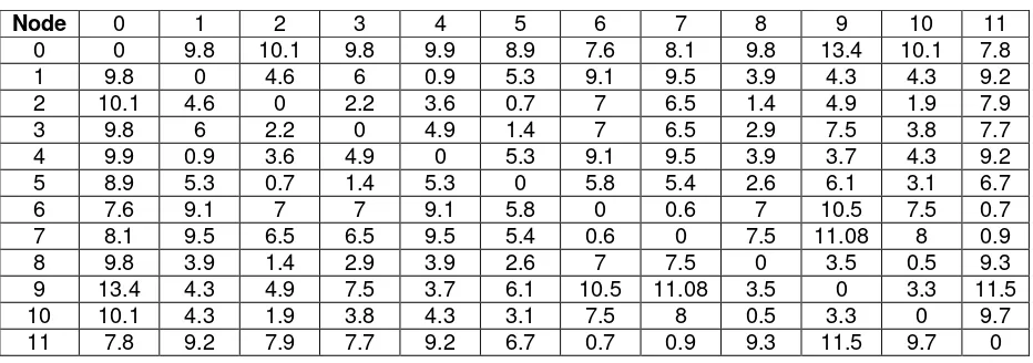
Suppose we have a graph that consists of a depot of softdrink industry and 12 customer points to serve. The cost matrix for the graph is given in Table 1, while the delivery and pick-up demands are given in Table 2. It is assumed that there is a homogeneous fleet of vehicles with capacities equal to 35 units. Since the total delivery demands is 84 and the total pick-up demands is 94, we need at least 3 vehicles to serve all customers.

With respect to the difference between pick-up and delivery demands, node 9, 1, and 3 are chosen as the seed nodes, while the rest are defined as the free nodes. Let node 9 be the first seed chosen to build the route, so

(4)

the maximum value of Z2(i,u,j), to the current

partial route. We now have R=(0, 9, 8, 12, 0) with L(0) = Cd(R) = 22; L(9) = 26; L(8) = 28;

and L(12) = 27. The next free node to be inserted is node 10 so that we have R=(0, 9, 8, 12, 10, 0) with L(0) = Cd(R) = 29; L(9) = 33;

L(8) = 35; L(12) = 34, and L(10) = 34.

Next, insert node 4 to the current partial route, so that we have R=(0, 9, 8, 12, 10, 4, 0) with L(0)=Cd(R)=37 which is exceeding

the vehicle’s capacity. Hence, drop node 4

from the route. The feasible route of the first vehicle is then R=(0, 9, 8, 12, 10, 0) with the associated travel cost of 31.7.

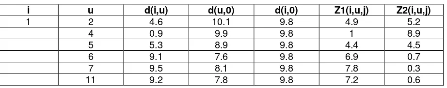
In a similar way as for the first vehicle, we now have Table 4 for the second vehicle that gives the feasible vehicle’s route of R=(0, 1, 4, 2, 5, 0). The associated travel cost of the second route is 23.9. Finally, we have Table 5 for the third vehicle. There are two feasible

vehicle’s routes, i.e. R=(0, 3, 7, 6, 11, 0) with the associated travel cost of 25.4 and R=(0, 3, 6, 7, 11, 0) with the associated travel cost of 26.1. We then choose the first alternative route to be the route of the third vehicle. Therefore, the total travel cost incurred by the fleet of the three vehicles is then 81.

Table 1. The Cost Matrix

Node 0 1 2 3 4 5 6 7 8 9 10 11

0 0 9.8 10.1 9.8 9.9 8.9 7.6 8.1 9.8 13.4 10.1 7.8

1 9.8 0 4.6 6 0.9 5.3 9.1 9.5 3.9 4.3 4.3 9.2

2 10.1 4.6 0 2.2 3.6 0.7 7 6.5 1.4 4.9 1.9 7.9

3 9.8 6 2.2 0 4.9 1.4 7 6.5 2.9 7.5 3.8 7.7

4 9.9 0.9 3.6 4.9 0 5.3 9.1 9.5 3.9 3.7 4.3 9.2

5 8.9 5.3 0.7 1.4 5.3 0 5.8 5.4 2.6 6.1 3.1 6.7

6 7.6 9.1 7 7 9.1 5.8 0 0.6 7 10.5 7.5 0.7

7 8.1 9.5 6.5 6.5 9.5 5.4 0.6 0 7.5 11.08 8 0.9

8 9.8 3.9 1.4 2.9 3.9 2.6 7 7.5 0 3.5 0.5 9.3

9 13.4 4.3 4.9 7.5 3.7 6.1 10.5 11.08 3.5 0 3.3 11.5

10 10.1 4.3 1.9 3.8 4.3 3.1 7.5 8 0.5 3.3 0 9.7

11 7.8 9.2 7.9 7.7 9.2 6.7 0.7 0.9 9.3 11.5 9.7 0

Table 2. The Delivery and Pick-up Demands

Demand Node

1 2 3 4 5 6 7 8 9 10 11 12

Delivery 7 8 6 8 6 7 8 7 6 7 5 9

Pick-up 10 9 9 7 5 5 8 9 10 7 7 8

Table 3. The Value of Z1(i,u,j) and Z2(i,u,j) for Vehicle-1

i u d(i,u) d(u,0) d(i,0) Z1(i,u,j) Z2(i,u,j)

9 2 4.9 10.1 13.4 1.6 8.5

4 3.7 9.9 13.4 0.2 9.7

5 6.1 8.9 13.4 1.6 7.3

6 10.5 7.6 13.4 4.7 2.9

7 11.08 8.1 13.4 5.78 2.32

8 3.5 9.8 13.4 -0.1 9.9

10 3.3 10.1 13.4 0 10.1

11 11.5 7.8 13.4 5.9 1.9

(5)

1 2 4.6 10.1 9.8 4.9 5.2

4 0.9 9.9 9.8 1 8.9

5 5.3 8.9 9.8 4.4 4.5

6 9.1 7.6 9.8 6.9 0.7

7 9.5 8.1 9.8 7.8 0.3

11 9.2 7.8 9.8 7.2 0.6

3 6 7 7.6 9.8 4.8 2.8

7 6.5 8.1 9.8 4.8 3.3

11 7.7 7.8 9.8 5.7 2.1

5. CONCLUSION

This paper has dealt with the vehicle routing problem that is frequently encountered in the distribution system of beverage industry, where the delivery of full bottles from the depot and the pick-up of empty bottles from the customers are performed simultaneously. Each customer can only be visited once by a vehicle without ever exceeding the vehicle capacity. To find the optimal solution of the problem, an integer programming model was developed based on the general assignment model of Fisher and Jaikumar. Since the optimization model can only solve relatively small problems, a heuristic algorithm, called the insertion procedures was also developed to solve the model more efficiently.

REFERENCES

1. Angelelli, E., Mansini, R. (2002). “The vehicle routing problem with time windows and simultaneous pick-up and delivery” in Quantitative Approaches to Distribution Logistics and Supply Chain Management, Klose, A., Speranza, M. G., Van Wassenhove, L. N. (Eds.), Springer, Berlin, 249-267.

2. Dethloff, J. (2001). “Vehicle routing and reverse logistics: The vehicle routing problem with simultaneous delivery and

pick-up”, Operations Research

Spectrum, 23:79–96.

3. Fisher, M. & Jaikumar, M. (1981). “A Generalized Assignment Heuristic for Vehicle Routing”, Networks, 11, 109-124.

4. Gribkovskaia, I., Halskau, Ø.,

Myklebost, K.N.B. (2001). “Models for pick-up and deliveries from depots with lasso solutions” In Proceedings of the 13th Annual Conference on Logistics Research NOFOMA 2001, Stefansson, G., Tilanus, B. (Eds.), Chalmers University of Technology, Göteborg, 279-293.

5. Min H. (1989). “The multiple vehicle routing problem with simultaneous

delivery and pickup points”,

Transportation Research 23A, 377–386.

6. Solomon, M.M. (1987), “Algorithms for

the Vehicle Routing and Scheduling

Problems with Time Window

Constraints”, Operations Research 35,

254265.

7. Tang, F.A. and Galvao, R.D. (2002).

“Vehicle routing problems with

simultaneous pick-up and delivery service”, Operations Research 39, 19– 33.

(6)