THESIS – SS 142501
POPULATION ANALYSIS OF DISABLED
CHILDREN BY DEPARTMENTS IN FRANCE
DIAH MEIDATUZZAHRA NRP 1314 201 003
ADVISORS Nicolas Pech Amélie Etchegaray
MASTER PROGRAM
DEPARTMENT OF STATISTICS
FACULTY OF MATHEMATICS AND NATURAL SCIENCES SEPULUH NOPEMBER INSTITUTE OF TECHNOLOGY SURABAYA
ANALYSE DE LA POPULATION
DES ENFANTS HANDICAPE
PAR DEPARTEMENT EN FRANCE
Réalisé par : Diah MEIDATUZZAHRA
Encadrant CREAI : Amélie ETCHEGARAY
Encadrant universitaire : Nicolas PECH
Rapport de stage
M2 MASS POP
Aix-Marseille Université
2015 /2016
DOCUMENT FOR SEPULUH NOPEMBER INSTITUTE OF TECHNOLOGY (ITS), INDONESIA
iii
POPULATION ANALYSIS OF DISABLED CHILDREN
BY DEPARTMENTS IN FRANCE
Name : Diah Meidatuzzahra
NRP : 1314 201 003
Advisors : Nicolas Pech Amélie Etchegaray
ABSTRACT
In this study, a statistical analysis is performed by model the variations of the disabled about 0-19 years old population among French departments. The aim is to classify the departments according to their profile determinants (socioeconomic and behavioural profiles). The analysis is focused on two types of methods: principal component analysis (PCA) and multiple correspondences factorial analysis (MCA) to review which one is the best methods for interpretation of the correlation between the determinants of disability (independent variable). The hierarchical cluster analysis (HCA) can be used to classify the departments according to their profile determinants. Analysis of variance or ANOVA is performed to know difference the between cluster and within cluster variances of two proxy data (AEEH and EN3-EN12). The PCA reduces 14 determinants of disability to 4 axes, keeps 80% of total information, and classifies them into 7 clusters. The MCA reduces the determinants to 3 axes, retains only 30% of information, and classifies them into 4 clusters. The ANOVA of the proxy data by department cluster are difference significant between cluster and the variance within of cluster is not difference significant, the cluster are homogeneous.
iv
ACKNOWLEDGEMENTS
In the name of Allah SWT, the beneficent and merciful. All praise is merely to The Mightiest Allah SWT, for the gracious mercy and tremendous blessing that enable me to accomplish this script. This research report entitled “Population Analysis of Disabled Children by Departments in France”, is submitted to fulfill one of the requirements in accomplishing the S-2 Degree Program at the Department of Statistics, Faculty of Mathematics and Natural Sciences, Sepuluh Nopember Institue of Technology, Surabaya (ITS).
There are many individuals who have generously suggested to improve this research report. First of all the writer would like to express his sincere gratitude and respect to his first advisor, Nicolas Pech and Amélie Atchegaray, who have contributed and given their valuable evaluations, comments, and suggestions during the completion and accomplishing of this research report. The writer also would like to express his deepest gratitude and respect to all professor of MASS Aix-Marseille Univercity (AMU) and the associate of CREAI PACA et Corse. And then, to coordinator of master program in statistics ITS, Dr.rer.pol Heri Kuswanto, thank you for supporting me to study abroad.
Last but not least, special gratitude and indebtedness are dedicated to beloved mother, Suhartini and beloved father, M. Syuhairi, and also all of family, who always give their loves, prayers, supports, and encouragements for every single path the writer chooses. Special thankfullness is also due to beloved friends, Statistics ITS 2014, the colleagues of MASS POP AMU 2015, and PPI (Perhimpunan Pelajar Indonesia) in Marseille, for their loves, prayers and supports.
Hopefully, this script would give a positive contribution to the educational development or those who want to carry out further research.
Surabaya, January 2017
v
II CONTEXT and PRESENTATION of DATA ... 3
2.1CREAI... 3
2.2The Project “Geography of the disabled population” ... 4
2.3The Determinants of DIsability ... 5
2.3.1The Professional category of social ... 5
2.3.2The education level of their parents ... 5
2.3.3The premature rate ... 6
2.3.4The Tax of Revenus ... 6
2.3.5The consumption of alcohol... 6
2.3.6The facilities and services of medical social for disabled ... 6
2.4 The Data of Proxy ... 7
2.1.1The AEEH data ... 7
2.1.2The EN3-12 data ... 7
III TRAITEMENTS of STATISTICS ... 8
3.1. Principal Components Analysis (PCA) ... 9
3.1.1 The Correlation Matrix ... 9
3.1.2 The Eigenvalue of the Correlation Matrix ... 10
3.1.3 Variables Results ... 11
3.1.4 The Departments Results ... 12
3.1.5 Conclusion of PCA ... 14
vi
3.2.1 Hierarchical Ascending Classification ... 15
3.2.2 Analysis of Variance ... 19
3.3. Strong Contribution of Certain Departments ... 26
3.3.1 Multiple Component Analysis (MCA) ... 26
3.3.2 Hierarchical Ascending Classification ... 29
3.3.3 Analysis of Variance ... 31
IV SUMMARY OF RESULTS ... 36
V CONCLUSION... 37
REFERENCES ... 38
ATTACHEMENTS... 43
vii
LIST OF TABLES
Table 2.1 The position of CSP ... 5
Table 2.2 The classify of education level... 6
Table 3.1 Correlation matrix ... 10
Table 3.2 The eigenvalues of the correlation matrix ... 10
Table 3.3 The average of axis ... 16
Table 3.4 ANOVA of between classes AEEH ... 19
Table 3.5 ANOVA of 6 classes ... 20
Table 3.6 ANOVA of within classes AEEH ... 22
Table 3.7 ANOVA of between 7 classes EN3-12 ... 23
Table 3.8 ANOVA of between 6 classes EN3-12 ... 24
Table 3.9 ANOVA of within 7 classes EN3-12 ... 25
Table 3.10 The identification labels of determinants variables ... 27
Table 3.11 The contribution of determinants variables ... 28
Table 3.12 The average of classes by axe ... 30
Table 3.13 ANOVA of MCA between classes AEEH ... 32
Table 3.14 ANOVA of MCA within classes AEEH ... 33
Table 3.15 ANOVA of MCA between classes EN3-12 ... 34
viii
LIST OF DIAGRAM
Diagram 3.1 Eigenvalue ... 11
Diagram 3.2 The contribution of determinants ... 12
Diagram 3.3 Representation of departments on axis 1and 2... 13
Diagram 3.4 Representation of departments on axis 3 and 4 ... 14
Diagram 3.5 The criteria of class number (PCA) ... 16
Diagram 3.6 Box Plot of 7 classes AEEH ... 20
Diagram 3.7 Box Plot of 6 classes AEEH ... 21
Diagram 3.8 Box Plot of classes 7 EN3-12 ... 23
Diagram 3.9 Box Plot of 6 classes EN3-12 ... 24
Diagram 3.10 The criteria of class number (MCA) ... 29
Diagram 3.11 Box Plot of 4 classes AEEH ... 32
ix
LIST OF ATTACHEMENTS
Attachments 1 Representation of variables on axes 1 et 2 ... 43
Attachments 2 Representations of variables on axes 3 et 4 ... 43
Attachments 3 Analyse of classifications on PCA - HAC ... 44
Attachments 4 Student test of Tukey (HSD) in AEEHdata ... 45
Attachments 5 Students Test of modulus maximum (GT2) on AEEH data ... 46
Attachments 6 T Tests of Bonferroni (Dunn) in AEEH ... 47
Attachments 7 Proc univariate residual of 7 Classe AEEH ... 48
Attachments 8 Distribution and Courbe Q-Q of absolut residuals on AEEH ... 49
Attachments 9 Plot of absolut residuals on AEEH ... 50
Attachments 10 Student Test of Tukey (HSD) on EN-12... 51
Attachments 11 Test modulus maximum (GT2) on EN3-12 ... 52
Attachments 12 T Tests of Bonferroni (Dunn) on EN3-12... 53
Attachments 13 Proc univariate of 7 Classe EN3-12 ... 54
Attachments 14 Distribution eand Courbe Q-Q of absolut residuals on EN3-12 ... 55
Attachments 15 Plot of absolut residuals on EN3-12 ... 56
Attachments 16 The inertie of MCA ... 57
Attachments 17 The Individuals and variables on axes 1 and 2 ... 58
Attachments 18 The Individuals and variables on axes 1 and 3 ... 55
Attachments 19 The Individuals and variables on axes 2 and 3 ... 59
Attachments 20 Analyse of classifications ... 60
Attachments 21 Classification of MCA ... 61
Attachments 22 Test of Tukey (HSD) sur taux_AEEH ... 63
Attachments 23 Test of modulus maximum (GT2) on AEEH ... 63
Attachments 24 T Tests of Bonferroni (Dunn) on AEEH... 64
Attachments 25 Proc univariate residual of 4 Classe AEEH ... 64
Attachments 26 Distribution and Courbe Q-Q of absolut residuals on AEEH ... 65
x
Attachments 28 Test of Tukey (HSD) on EN3-12 ... 67
Attachments 29 Test of modulus maximum (GT2) on EN3-12 ... 67
Attachments 30 T Tests of Bonferroni (Dunn) on EN3-12... 68
Attachments 31 Proc univariate residuals of 4 Classe EN3-12... 68
Attachments 32 Distribution and Courbe Q-Q of absolut residuals on EN3-12 ... 69
Attachments 33 Plot of absolut residuals on EN3-12 ... 70
1
I. INTRODUCTION
The term “disability” is defined as a limitation of a person's ability to interact with their environment, due to a permanent disability or non-permanent that leads to stress and moral disorder, intellectual, physical or social. Disability is the consequence of an impairment that may be physical, cognitive, mental, sensory, emotional, developmental, or some combination of these. A disability may be present from birth, or occur during a person's lifetime. Disability comes in multiple forms and ambiguous definition. It is to be distinguished from the disease or the accident, which can be the disability origin.
In France, the definition disability is governed by French law dated 11 February 2005 on the opportunities and the same rights, and the participation and
citizenship of disability people, that “Disability of activity limitations or
restrictions on participation in the social life suffered by a person, due to
substantial continuing modification of one or more functions”.
One of the institutions cared for the disabled is CREAI branch PACA et Corse. CREAI collaborated with Population Environment Development Laboratory (LPED) Aix-Marseille University propounds a project "Geography of Disability". The purpose is to estimate of the population and establishment medical social service. Therefore, statistical analysis is required to estimate the disabled population of multiple databases which were defined as disability determinants.
2
3
II. CONTEXT AND PRESENTATION of DATA
2.1 Centre inter-Régional d’Etudes, d’Action et d’Information (CREAI)
CREAI PACA et Corse or Central interregional of studies, action and information branch Provence-Alpes-Côte d'Azur (PACA) and Corse in France was founded in 1965 and belongs to the National Association of CREAI (ANCREAI) for a person with the condition of vulnerability. The CREAI is a private organizations and non-profit status established by statute law in 1901 which is subsidized by the State to optimize information sharing, collaboration and develop synergies of the technical experts to reflection and observation in the sectors of social action and medico-social.
The main tasks entrusted to the Creai include:
- Observation of the needs and expectations of populations
- The carrying out of studies and observations on the specific phenomena centered of disability (Regional Health Agency), in the region or the departments
- Technical expertise through the internal evaluation of actions (accompanying the internal evaluation of institutions and medico-social services through training actions)
- Training professionals on topics such as violence, wellness, personalized project
- Animation notably to facilitate exchanges between the actors concerned by a thematic, but also in order to improve collaborations and encourage innovations
4 The team names of CREAI workers:
DIRECTION - Serge DAVIN (President)
- Dr Monique PITEAU-DELORD (Directress)
Studies-Observations-Expertise - Sophie BOURGAREL (Technical Advisor)
- Céline MARIVAL (Technical Advisor)
- Amélie ETCHEGARAY (Technical Advisor)
- Philippe PITAUD (Scientific
FORMATION - Hélène CATTANEO
- Emilie GIRARD (Secretariat of the training center)
ADMINISTRATION - Christiane CHAZOT (Executive
Management)
INFORMATICS SERVICE - Benjamin CAYRE (Computer
scientist)
2.2 The Project "Geography of the disabled population”
CREAI collaborated with Population Environment Development
5
of Disability" between 0 and 59 years by 96 departments in France. The purpose is
to estimate of the population and establishment medical social service.
2.3 The Determinants of Disability
The hypothesis of the project "Geography of Disability" is the distribution unusual of the disabled population in the region. The distribution of this population related by multiple factors, for example, economic factors, education, environment, lifestyle, etc., called the determinants of disability. Six groups of determinants identified:
2.3.1 The professional category of social (CSP)
The CSP based on the data of INSEE. Labor force of 15 years and more having a job by gender, age, and the CSP are divided into 6 positions, is show on table 2.1.
Table 2.1. The position of CSP
Number The professional category of social
1. Farmer
2. Artisan, craftsman and trader 3. Manager and high professions 4. Intermediate professions
5. Employee
6. Labor
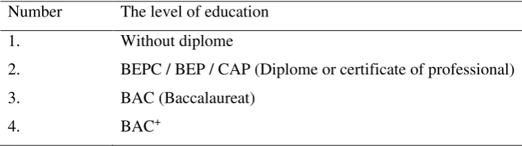
2.3.2 The education level of their parents
6
Table 2.2. The clusterify of education level Number The level of education
1. Without diplome
2. BEPC / BEP / CAP (Diplome or certificate of professional)
3. BAC (Baccalaureat)
4. BAC+
2.3.3 The Premature Rates
The EPIPAGE study showed the importance of disabling sequelae preterm infants, before 33 weeks of amenorrhea (WA), and among those born between 33 and 36 WA of age. According EPIPAGE, if the preterm birth is increased, the risk of disability is also. The 8th day certificate (Cs8) data used as database from 2010 to 2012.
2.3.4 The Tax of Revenues
The report of revenues tax is derived from local INSEE Social and Tax File (Philosophy) data. The first quartile of income report is the average wage in the department below which is 25% of wages (CREAI,2010).
2.3.5 The Consumption of Alcohol
The consumption of alcohol among women is unknown, therefore the number of premature deaths due to overdose of alcohol (it cause alcoholic psychoses and alcoholic cirrhosis of the liver) in women under the 65 years old were selected.
2.3.6 The facilities and services of medical social for disabled
7
1000 children and also the Orne (18 places for 1000 children) and the Creuse (17 places for 1000 children).
2.4 The data of Proxy
The proxy data is concern and count of the population with a disability in France. Two databases are considered to be proxy data for children, namely the number of beneficiaries of the Allowance for the Education of Handicapped Children (AEEH) and the number of disabled children enrolled in national education (EN3-12).
2.4.1 The data of the Allowance for the Education of Handicapped Children
(AEEH)
The AEEH is designed to help parents who assume the responsibilities of disabled children, regardless of their resources. It is awarded to families with disabled children who have a disability rate recognized by the Commission for the Rights and Autonomy of Persons with Disabilities (CDAPH) within the Departmental Houses for Persons with Disabilities (MDPH). According to the socioprofessional category of the household, the AEEH can be paid by the Caisse d'Allocation Familiale (CAF), the Mutuelles Sociale Agricole (MSA) and the Régime Social des Indépendants (RSI).
2.4.2 Survey No. 3 and 12 on the enrollment of pupils with disabilities in
primary and secondary education (EN 3-12)
9
III. TRAITEMENT OF STATISTICS
The aim of this section is to determine, using Principal Component Analysis (PCA) and hierarchical ascending clusterification (HCA), groups of departments with the same determinant profiles (socio-economic and behavioral profiles ) And to know the « between » and « within » of cluster variances on the proxy by analysis of variances (ANOVA). If certain departments have too much contribution, it will be necessary to go through a factor analysis of multiple correspondences (MCA) and apply the same methodology (HCA and ANOVA).
10 3.1 Principal Components Analysis (PCA)
A principal component analysis (PCA) is concerned with explaining the variance-covariance structure of a set of variables through a few linear combinations of these variables. PCA is a statistical procedure that uses an orthogonal transformation to convert a set of observations of possibly correlated variables into a set of values of linearly uncorrelated variables called principal components. Its general objectives are reduction and interpretation of dimension (axes) data without reducing significantly the characteristics of the data. PCA is also often used to avoid problems of multicollinearity between independent variables in a multiple regression model.
The number of principal components is less than or equal to the number of original variables. This transformation is defined in such a way that the first principal component has the largest possible variance (that is, accounts for as much of the variability in the data as possible), and each succeeding component in turn has the highest variance possible under the constraint that it is orthogonal to the preceding components. The resulting vectors are an uncorrelated orthogonal basis set. PCA is sensitive to the relative scaling of the original variables.
As part of this process, the PCA is involved in the interpretation of the relationship between the determinants of disability, interdependent variables. Its main purpose is to condense the information given by the determinants into a smaller number of independent fundamental variables that can not be directly observed.
3.1.1 The Correlation matrix
11
Table 3.1 Correlation matrix
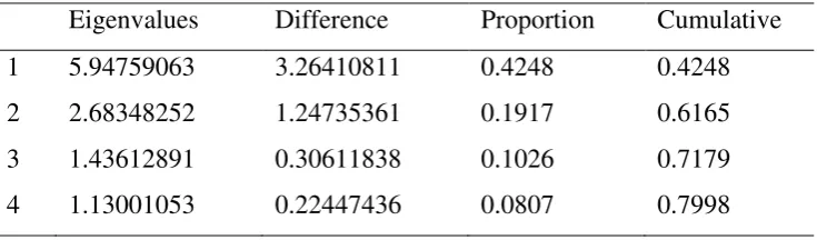
3.1.2 The Eigenvalue of the Correlation Matrix
Table 3.2 and diagram 3.1 below provide the inertia of each axis. By looking at the eigenvalues and especially that greater than 1 then axis is selected four. The first axis contains 42% of the diversity from the original data with eigenvalue is 5.95. The second axis allows to restore 19% of the total inertia with eigenvalue is 2.68. The third axis contains 10% of the information and the fourth 8%. These four axis thus make it possible to retain 80% of the information (Rule of Kaiser).
Table 3.2 The eigenvalues of the correlation matrix
Eigenvalues Difference Proportion Cumulative
1 5.94759063 3.26410811 0.4248 0.4248
2 2.68348252 1.24735361 0.1917 0.6165
3 1.43612891 0.30611838 0.1026 0.7179
12
Diagram 3.1 Eigenvalue
3.1.3 Variables Results
Diagram 2 allows analyzing the contribution of the variables to the axek ( ). It is comparing the absolute value of variables with:
1
√𝑃 (3.1)
Where ,
𝑝 = 14
The higher values corresponded to the variables which most contribute formation of the axis. The positive or negative symbol is showed high or low contribution of variable.
The first axis is correlated positive with the labor variable and the level of education without a diploma, BEPC, CAP or BEP. Conversely, it is negative correlation with the manager variable as well as the level of education with a diploma above the bac. The second axis is contrasts with the rate of artisans-craftsmen-traders and the education level of people with the baccalaureate and the rate of preterm, the rate of consumption of alcohol and the rate of workers.
13
Diagram 3.2 The contribution of determinants
3.1.4 The Departments Results
The ACP also calculated the coordinates of the individuals on the axes and their contributions to the dispersion according to each of these axes with the formula :
(3.2) Where, = eigenvalue
14
for the Creuse (23). The departments of Haute Garonne (31), Rhone (69), Hauts de Seine (92), Yvelines (78), Val de Marne (94) and Essonne (91) have coordinates less than -4.
Five departments have large contributions 4% and account for almost 46% of the variance: They are predominant in the definition of axis 1. The 5 departments are Paris (75) with 16% contribution, Hauts de Seines (92) 12%, Les Yvelines (78) 9%, Haute Garonne (31) 5% and the Rhone (69) 4%.
Diagram 3.3 Representation of departments on axis 1and 2
15
(93) with 9%; The Haute Savoie (74) with 6% and the Hauts de Seine (92) with 5%. Details can be found in the diagram below.
Diagram 3.4 Representation of departments on axis 3 and 4
3.1.5 Conclusion of PCA
16
3.2 The Balanced Contribution of departments
3.2.1 Hierarchical Cluster Analysis (HCA) of the departments using the
axes of the PCA
A hierarchical cluster analysis method is a procedure which represents the data as a nested sequence of partitions. An example of the corresponding proposed to determine the best cutting point, to automatically find the number of clusters [mil88].
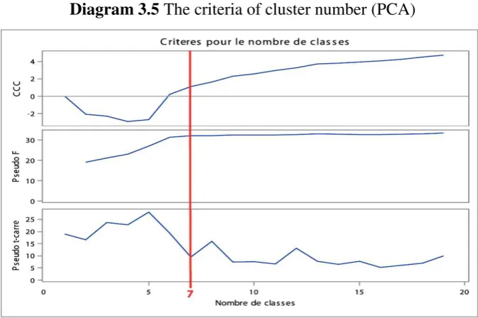
A. The choice of the number of clusters
The number of clusters is selected by three criteria. The diagram below represents the Cubic Clastering Criterion (CCC), pseudo F and pseudo t2 as a function of the number of clusters.
The Cubic Clustering Criterion (CCC)
CCC values greater than 2 indicate good classification. The peak in the CCC between 0 and 2 indicate is a possible classification.
The Pseudo F
As a general rule, the higher this statistic, the better the score.
The pseudo t²
17
Diagram 3.5 The criteria of cluster number (PCA)
The number of clusters is must satisfied above the criteria. The seven clusters are selected of departments.
b. The Characterization and localization of clusters
The table 3.3 below is showed the average of axis in each cluster. Table 3.3 The average of axis
The characterization of the seven clusters is as follows:
Cluster 1
18
Maritime, Charente, The Haute Vienne, the Dordogne, the Corrèze, the Puy de Dôme, the Haute Loire, the Ardèche, the Drome, the Landes, Lot and Garonne, Tarn, Tarn et Garonne Pyrenees and the Ariège.
Cluster 2
Cluster 2 is composed mainly of the inverse of axis 1 of the PCA, i.e. a high rate of executives as well as a rate of people with a diploma superior to the bac. The positive average 0.83 of the axis 4 corresponds to a population having mainly as a level of education the patent, CAP or BEP, a high level of intermediate professions and a first quartile of the median income. This cluster regroups 18 départements spread all over France. These include Ain, Côte-d'Or, Finistère, Haute-Garonne, Gironde, Ille-et-Vilaine, Indre-et-Loire, Isère, Loire-Atlantique, Pyrénées-Atlantiques, Rhône, Savoie, Haute-Savoie, Seine-et-Marne, Yvelines, Essonne, Val-de-Marne and Val-d Oise.
Cluster 3
Cluster 3 includes all the departments of the Mediterranean arc (Hautes Alpes, Alpes-de-Haute-Provence, Alpes-Maritimes, Vars, Bouches-du-Rhône, Vaucluse, Gard, Hérault, Aude, Pyrénées-Orientales Corsica "Corse-du-Sud and Haute-Corse"). They are characterized by a negative mean for axis 2. This means that these are departments composed of people with a tray level and a craftsman status. The mean of 1.34 of axis 3 means that this region is also characterized by a high level of intermediate and employee professions and alcohol consumption.
Cluster 4
19
and Maine et Loire) East of France (the Meurthe et Moselle, the Lower Rhine and the Upper Rhine, the Vosges, the Territoire de Belfort and the Doubs).
Cluster 5
Cluster 5 consists mainly of axis 1, that is, a population without a diploma or a BEPC, CAP, BEP or a baccalauréat. The dominant CSPs are the working clusters. These departments are mainly located in the Massif Central: Aveyron, Cantal, Creuse, Lot and Lozère. The Gers is also attached to this cluster.
Cluster 6
Cluster 6 is the cluster of workers, employees and intermediate professions who do not have a diploma or the BEPC, CAP or BEP. The rate of premature deaths related to alcohol is high as premature births. The departments are located in the Nord Pas de Calais region and its surroundings (Somme, Aisne and Ardenne and Aube). The Seine Saint Denis also belongs to this cluster.
Cluster 7
Cluster 7 consists of only two departments: Paris and the Hauts de Seine. These are departments represented by an extreme average of the inverse of axis 1: a population with a level of education higher than the bac and a socio-professional category of executives.
B. Conclusion Ascending Hierarchical Clustering (HCA)
The Hierarchical Ascending Clustering (HCA) issued by the PCA made it possible to group the departments into 7 clusters. With 35 departments, cluster 1 is the cluster with the most individuals. On the contrary, cluster 7 contains only two.
20 3.2.2 Analysis of Variance (ANOVA)
Analysis of Variance (ANOVA) is a statistical method used to analyze the differences among group means and their associated procedures (such as "variation" among and between groups).
In the case study, ANOVA is performed to the difference of variable disabled determinants in proxy data (AEEH and EN3-12) by the clustering of departments (between and within cluster).
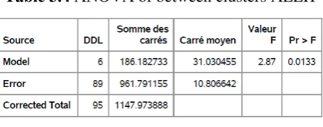
A. ANOVA of the data AEEH
Analysis Between Clusters
On the basis of the HCA analysis, ANOVA is performed to difference between the 7 clusters on the AEEH data. The hypothesis is:
𝐻0: 𝜇1 = 𝜇2 = ⋯ = 𝜇𝑘 ; 𝑤ℎ𝑒𝑟𝑒 𝑘 = 𝑡ℎ𝑒 𝑛𝑢𝑚𝑏𝑒𝑟 𝑜𝑓 𝑐𝑙𝑢𝑠𝑡𝑒𝑟 (1, 2, 3, 4, 5, 6, 7)
(There is no significant difference between the averages of the 7 clusters)
𝐻1: At least one 𝜇𝑖 ≠ 𝜇𝑘 ; 𝑤ℎ𝑒𝑟𝑒 𝑖 = 1,2, … , 𝑘
(At least one significant difference between the averages of the 7 clusters)
Table 3.4 ANOVA of between clusters AEEH
In the table 3.4, the value of probability Pr> F = 0.0133 is less than . The hypothesis is rejected, so, at least a significant difference between the averages of the 7 clusters of the AEEH data.
21
difference between the averages. But the Tukey method is revealed significant differences between clusters 6 and 4 and clusters 6 and 7.
As a reminder, clusters 4 and 6 are characterized by a high rate of premature births and consumption of alcohol, the workers, artisan and agricultural clusters. Cluster 6 is also characterized by a low ESMS rate and the lowest quartile of tax revenue. On the contrary, cluster 7 comprises only two departments, Paris and Hauts de Seine, departments with a population of the graduate level.
Diagram 3.6 Box Plot of 7 clusters AEEH
In box-plot diagram 3.6, the distribution of cluster 7 is very different from other clusters. Only two departments in cluster 7, Paris and the Hauts de Seine, departments already very different at the socio-economic level.
Therefore, a new ANOVA is realized on the 6 clusters by dismissing the cluster 7. The hypothesis is :
𝐻0: 𝜇1 = 𝜇2 = ⋯ = 𝜇𝑗 ; 𝑤ℎ𝑒𝑟𝑒 𝑘 = 𝑡ℎ𝑒 𝑛𝑢𝑚𝑏𝑒𝑟 𝑜𝑓 𝑐𝑙𝑢𝑠𝑡𝑒𝑟 (1, 2, 3, 4, 5, 6)
(There is no significant difference between the averages of the 6 clusters)
𝐻1: At least one 𝜇𝑖 ≠ 𝜇𝑗 ; 𝑤ℎ𝑒𝑟𝑒 𝑖 = 1,2, … , 𝑗
22
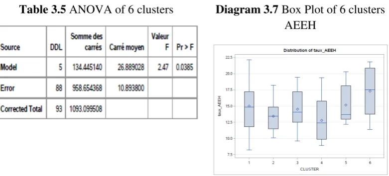
Table 3.5 ANOVA of 6 clusters Diagram 3.7 Box Plot of 6 clusters AEEH
In table 3.5 ANOVA, the significant value is 0.0385 and allows us to reject H0 for a significance level of 5%. The tests of Bonferroni, Tukey and Hochberg-GT2 showed the same result: there is a significant difference in the means of clusters 6 and 4.
The values of F on the anova 7 clusters and the anova 6 clusters are both significant and less than α = 5%. In other words, cluster 7 which consists of two departments (Paris and the Hauts de Seine) does not influence the average differences between the other clusters.
Analysis Within Clusters
The ANOVA within clusters is done from the residual or error data of the previous ANOVA model. Before analyzing this data, test the normality of the data performed by univariate analysis. The following assumptions:
H0: Data is a normal distribution H1: Data is not normal distribution
23
absolute values of the residuals between the 7 clusters on the AEEH data intra-cluster ANOVA. The following assumptions:
𝐻0: 𝜎1 = 𝜎2 = ⋯ = 𝜎𝑘 ; 𝑤ℎ𝑒𝑟𝑒 𝑘 = 𝑡ℎ𝑒 𝑛𝑢𝑚𝑏𝑒𝑟 𝑜𝑓 𝑐𝑙𝑢𝑠𝑡𝑒𝑟 (1, 2, 3, 4, 5, 6, 7)
(There is no significant difference between the variances within of the 7 clusters)
𝐻1: At least one 𝜎𝑖 ≠ 𝜎𝑘 ; 𝑤ℎ𝑒𝑟𝑒 𝑖 = 1,2, … , 𝑘
(At least one significant difference between the variances within of the 7 clusters)
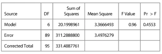
Table 3.6 ANOVA of within clusters AEEH
Table 3.7 of the ANOVA gives a value of and the probability that Pr> F = 0.4553 is greater than. It can’t reject H0, there is no significant difference in the variances within each of the 7 clusters. Moreover, it is supported by the Bartlette test which is also shows the value of P-value> 0.05 and ensures the homogeneity of the variances each of the 7 clusters.
B. ANOVA of the EN3-12 data
The second ANOVA is the analysis of variance by the number of children with disabilities in the national education (EN3 and EN12). First, analyze the mean difference between the 7 clusters and second step is analyze the difference of variance within each of these clusters on EN3-12 data.
Analysis Between Clusters
24
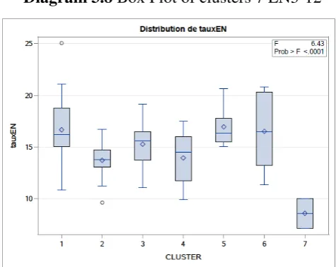
Table 3.7 ANOVA of between 7 clusters EN3-12
The Bonferroni, Hochberg-GT2 and Tukey tests are showed the same results: there is a significant difference between the averages of the following clusters: 5-7; 1-4; 1-2; 1-7; 6-7; and 3-7.
Diagram 3.8 Box Plot of clusters 7 EN3-12
In the diagram 3.8, the distribution of cluster 7 is very different from the other clusters. Therefore, as like as the AEEH, the 6 clusters is analyzed by discarding cluster 7, the hypothesis is thus:
𝐻0: 𝜇1 = 𝜇2 = ⋯ = 𝜇𝑗 ; 𝑤ℎ𝑒𝑟𝑒 𝑘 = 𝑡ℎ𝑒 𝑛𝑢𝑚𝑏𝑒𝑟 𝑜𝑓 𝑐𝑙𝑢𝑠𝑡𝑒𝑟 (1, 2, 3, 4, 5, 6)
(There is no significant difference between the averages of the 6 clusters)
𝐻1: At least one 𝜇𝑖 ≠ 𝜇𝑗 ; 𝑤ℎ𝑒𝑟𝑒 𝑖 = 1,2, … , 𝑗
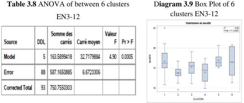
25 Table 3.8 ANOVA of between 6 clusters
EN3-12
Diagram 3.9 Box Plot of 6 clusters EN3-12
Table 3.8 of the ANOVA gives a value and the probability Pr> F = 0.0005 is less than α = 5%. The hypothesis is rejected; there is a significant difference between the averages of the number of children with disabilities in the national education according to the 6 clusters of the CAH.
The Bonferroni, Tukey and Hochberg-GT2 tests offer one common result: there is a significant difference in the averages of the rates of handicapped children enrolled in national education between grades 1-4 and 1-2.
• Analysis Within Clusters
As for the AEEH, before analyzing this data, test the normality of the data performed by univariate analysis. The Kolmogorov-Smirnov test will be able to show whether the data follow a normal distribution or not. The P-value of the Kolmogorov-Smirnov test is greater than α = 5% or 0.05 (P_Value:> 0.15), then it can’t reject H0, the data is a normal distribution.
And then, ANOVA is proceed to analyze the difference of the mean of the absolute values of the residuals between the 7 clusters on the EN3 and EN12 data. The following assumptions:
𝐻0: 𝜎1 = 𝜎2 = ⋯ = 𝜎𝑘 ; 𝑤ℎ𝑒𝑟𝑒 𝑘 = 𝑡ℎ𝑒 𝑛𝑢𝑚𝑏𝑒𝑟 𝑜𝑓 𝑐𝑙𝑢𝑠𝑡𝑒𝑟 (1, 2, 3, 4, 5, 6, 7)
(There is no significant difference between the variances within of the 7 clusters)
𝐻1: At least one 𝜎𝑖 ≠ 𝜎𝑘 ; 𝑤ℎ𝑒𝑟𝑒 𝑖 = 1,2, … , 𝑘
26
Table 3.9 ANOVA of within 7 clusters EN3-12
The table 3.10 of the ANOVA gives a value probability Pr> F = 0, 7563 is greater than. α = 5% or 0.05 H0 is not rejected, then there is no significant difference in the variances within each of the 7 clusters. Moreover, it is supported by the Bartlette test which also shows the value of P-value> 0.05 and ensures the homogeneity of the variances each of the 7 cluster.
C. Conclusion Analysis of variance (ANOVA)
27
3.3. Strong Contribution of Certain Departments
3.3.1 Multiple Component Analysis (MCA)
Multiple correspondence analysis (MCA) is the factorial method which adapted to tables. It is a set of individuals which described by several qualitative variables. It can be presented in many different ways. In France, following the work of L. Lebart, the most common is to focus on the similarities with correspondence analysis, a method designed to study the relationship between two qualitative variables. As a PCA, the aim of multiple component analysis (MCA) is to read the information contained in a multidimensional space by a reduction of the dimension. The MCA is permitted to answers the following questions:
- Which departments resemble each other? Which are different?
- Are there homogeneous groups of individuals? Is it possible to identify a typology of individuals?
A. Construction of the table data
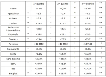
In this study, the clusterification of variable is selected into four clusters. The boundaries of the clusters being defined by the quartiles and renamed with readily identifiable labels as shown in Table 3.11 below.
28
Table 3.10 The identification labels of determinants variables
B. Eigenvalue and Numbers of Axis
The number of axis is determined by the formula :
(
𝑀𝑚
− 1)
(3.3)Where,
m = 14 disability determinant variables
M = 56 sum of the modalities of the active variables
By attachment 4, the eigenvalue is decided three axis with 30% of the total inertia.
C. Results on variables
29
Table 3.11 The contribution of determinants variables
The first axe is opposed the departments which manager have a the education level of bac and a first quartile of revenus tax, and the departments which workers without a diploma or a BEPC / CAP / BEP level. The second axe is defined the departments with artisan, craftsman and trader. The manager and the premature rates are low. On the contrary, the character of departments with a large population is not only manager but also workers, a first quartile of revenue tax and a high rate of premature.
The third axe is included the departments with a high rate of farmers, craftsmen and employees who do not have a high income quartile. The ESMS rate is poor too. On the other hand, the departments which is a large number of managers and intermediate professions with a higher or lower quartile of tax revenue and a high ESMS rate.
D. Results on the departments
30
coordinate. The MCA chart is difficult to interpret. The superposition of the 56 variables and the 96 departments do not allow the identification of departments.
E. Conclusion Multiple component analysis (MCA)
The MCA reduces the determinants to 3 axes, retains only 30% of total information. However, the determinant of the alcohol consumption does not contribute to these axes.
3.3.2 Hierarchical Cluster Analysis (HCA) of the departments using the
axes of the MCA
As previously, the hierarchical cluster analysis will classify the departments into homogeneous clusters.
A. The choice of the number of clusters
Diagram 3.10 The criteria of cluster number (MCA)
31
b. The Characterization and localization of clusters
The table 3.13 below is showed the average of axis in each cluster. Table 3.12 The average of clusters by axe
The characterization of the four clusters is as follows:
Cluster 1
Cluster 1 is consists mainly of axis 1 which a high rate of workers without a diploma or BEPC, BEP or CAP. There is little presence of senior or intermediate level professions at the Baccalaureate level. Cluster 1 is comprised 23 departments in the center and north of France: Haute-Marne, Mayenne, Meuse, Nièvre, Orne, Pas-de-Calais, Haute-Marne, Saône, Saône-et-Loire, Deux-Sèvres, the Ardennes, Vendée, Vosges, Yonne.
Cluster 2
Cluster 2 is composed to the axe 3 or regions with a population of managers and intermediate professions, some farmers and artisan, craftsman and trader. The first quartile of the revenue tax is a little high and the rate of equipment in ESMS also. Cluster 2 is the cluster which 31 departments in the northern of France except the Pyrénées Atlantiques (64).
Cluster 3
Alpes-32
de-Haute- Hautes-Pyrénées, Pyrénées-Orientales, Ardèche, Tarn, Tarn-et-Garonne, Var, Vaucluse, Ariège.
Cluster 4
Cluster 4 is the largest on axis 1. It is characterized by a large population of managers and intermediate professions with a higher education level of bac. Thus, the first quartile of tax revenue is strong. There are few employees, workers and farmers. The 19 departments are Paris and suburbs to Rennes, Nantes, Bordeaux, Toulouse, Montpellier, Nice, Lyon, Grenoble and Strasbourg.
C. Conclusion of Hierarchical Cluster Analysis (HCA)
The HCA issued by the MCA put the 96 departments into 4 clusters. In cluster 1, there are 23 departments and cluster 2 is the biggest cluster because there are 31 departments. Cluster 3 includes 23 departments and in cluster 4 only 19 departments.
3.3.3 Analysis of Variance (ANOVA) of proxies
Like ANOVA resulting from the HCA-PCA, an analysis of variance is carried out to determine the average differences in the AEEH and EN 3-12 data by the clusterification of departments (between and within cluster).
A. ANOVA of the data AEEH
Analysis Between Clusters
On the basis of the CAH analysis, ANOVA is performed to difference between the 4 clusters on the AEEH data. The hypothesis is:
𝐻0: 𝜇1 = 𝜇2 = ⋯ = 𝜇𝑛 ;
𝑤ℎ𝑒𝑟𝑒 𝑛 = 𝑡ℎ𝑒 𝑛𝑢𝑚𝑏𝑒𝑟 𝑜𝑓 𝑐𝑙𝑢𝑠𝑡𝑒𝑟 𝑜𝑛 𝑀𝐶𝐴 (1, 2, 3, 4)
(There is no significant difference between the averages of the 4 clusters)
𝐻1: At least one 𝜇𝑖 ≠ 𝜇𝑛 ; 𝑤ℎ𝑒𝑟𝑒 𝑖 = 1,2, … , 𝑛
33
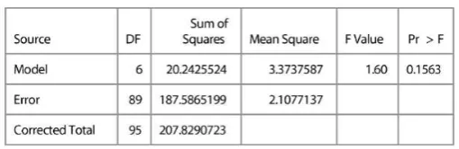
Table 3.13 ANOVA of MCA between clusters AEEH
In Table 3.14 the value of probability Pr> F = 0.0064 is less than . The hypothesis is rejected, so, at least a significant difference between the averages of the 4 clusters of the AEEH data. The Bonferroni, Tukey and Hochberg-GT2 tests offer a common result: there is a significant difference in the average of the beneficiary rates of the AEEH of clusters 1 and 2 and 1 and 4.
Diagram 3.11 Box Plot of 4 clusters AEEH
In diagram 3.11, the averages of each cluster are in the same rank. The clusters are not very different.
ANOVA analysis within clusters
The ANOVA analysis within clusters is done from the residual or error data of the previous ANOVA model. Before analyzing this data, test the normality of the data performed by univariate analysis. The following assumptions:
34
On the base of the univariate analysis, the Kolmogorov-Smirnov test will be able to show whether the data follow a normal distribution or not. The P-value of the Kolmogorov-Smirnov test is greater than α = 5% or 0.05 (P_Value:> 0.15), then it can’t reject H0, the data follow a normal distribution. And then, ANOVA is proceed to analyze the difference of the mean which the absolute values of the residuals between the 4 clusters on the AEEH data intra-cluster ANOVA. The following assumptions:
𝐻0: 𝜎1 = 𝜎2 = ⋯ = 𝜎𝑛 ;
𝑤ℎ𝑒𝑟𝑒 𝑛 = 𝑡ℎ𝑒 𝑛𝑢𝑚𝑏𝑒𝑟 𝑜𝑓 𝑐𝑙𝑢𝑠𝑡𝑒𝑟 𝑜𝑛 𝑀𝐶𝐴 (1, 2, 3, 4)
(There is no significant difference between the variances within each on the 4 clusters)
𝐻1: At least one 𝜎𝑖 ≠ 𝜎𝑛 ; 𝑤ℎ𝑒𝑟𝑒 𝑖 = 1,2, … , 𝑛
(At least one significant difference between the variances within of the 4 clusters)
Table 3.14 ANOVA of MCA within clusters AEEH
35 B. ANOVA of the EN3-12 data
Analysis Between Clusters
Like the AEEH data, table 3.16 is showed ANOVA enters cluster on data EN3-12 is rejects H0. The value P-value <0.0001 is less than a threshold of 5%.
Table 3.15 ANOVA of MCA between clusters EN3-12
The methods Bonferroni and Hochberg-GT2 tests are showed the same results: there is a significant difference between the averages of the following clusters: clusters 3 and 4, and clusters 1 and 4. The Tukey method is revealed significant differences between clusters 3 and 2, clusters 3 and 4, clusters 1 and 4.
Diagram 3.12 Box Plot of 4 clusters EN3-12
36 • ANOVA analysis within clusters
Table 3.16 ANOVA of MCA within clusters EN3-12
The table 3.16 of the ANOVA gives a value probability Pr> F = = 0, 8703 is greater than. α = 5% or 0.05 H0 is not rejected, then there is no significant difference in the variances within each of the 4 clusters. Moreover, it is supported by the Bartlette test which also shows the value of P-value> 0.05 and ensures the homogeneity of the variances each of the 4 cluster.
C. Conclusion Analysis of variance (ANOVA)
37
IV. SUMMARY OF RESULTS
Statistical analysis performed to model the variations of disabled children about 0-19 years old population among French department consisting of 14 determinant variables of children disabilities based on six categories, namely, the professional category of social (CSP) of their parents, the level education of their parents, the premature rates, the tax of revenues, alcohol consumption, facilities and services of medical social for disabled. The aim is to clusterify departments according to their profiles determinants (socioeconomic and behavioral profiles).
The PCA reduces 14 determinants of disability to 4 axes, keeps 80% of total information. PCA is also calculating the coordinates of the department and the contribution of the determinants variables per axis. It is not balanced because some departments have too strong contribution. The Hierarchical Ascending Clusterification (HCA) issued by the PCA made it possible to group the departments into 7 clusters. With 35 departments, cluster 1 is the cluster with the most individuals. On the contrary, cluster 7 contains only two. The different averages of the proxy data (AEEH and EN 3-12) issued HCA of PCA by department clusters are significantly different between clusters. On the contrary, the difference of variance within clusters is not significant. The groups are homogeneous. The best method to identify the two-average differences is Tukey. The Tukey test is generally more effective to testing a large number of pair’s averages.
38
39
V. CONCLUSION
41
REFERENCES
ACP sous SAS : http://www.univ-mrs.fr/~reboul/ACPsas.doc, consulté le 1er juin 2016.
Analyse factorielle multiple des correspondances (AFCM) :
http://www.math.univ-toulouse.fr/~besse/Wikistat/pdf/st-m-explo-afcm.pdf, le 1er juin 2016.
Baccini, A. (2010), Statistique descriptive multidimensionnelle, Publications de
l’institut de mathématiques de Toulouse, page 37.
Bressoux, P. (2010), Modélisation statistique appliquée aux sciences sociales, De boeck, 464p.
Dagnelie, P. (1975), Analyse statistique à plusieurs variables, Les presses agronomiques de gembloux, page 362.
Espagnacq M. (2015), Populations à risque de handicap et restrictions de participation sociale Dossiers solidarité et santé, Drees. n°68, page 18.
INSEE, The National Institute of Statistics and Economic Studies collects, analyses and disseminates information on the French economy and society
Laidier, L. (2015), A l'école et au collège, les enfants en situation de handicap constituent une population fortement différenciée scolairement et socialement. Note d'information DEPP n°4, page 4.
Le Centre interregional s’Etudes, d’Action et d’Informations (CREAI) en faveur des
personnes en situation de vulnérabilité
Mormiche, P. (2003), Handicap et Inégalités sociales. Revue française des affaires sociales 2003/1-2 (n° 1-2) , page11-29.
(2011) Organisation Mondiale de la Santé (OMS), France.
Pech, N., Les Guides SAS - L’analyse des données : La procédure cluster, Document du cours MASS POP, 2015/2016, page 160-252.
Rakotomalala, R. (2011), Tests de normalité Techniques empiriques et tests statistiques, Université Lumière Lyon, vers no.2, page 59.
Rican, S. (2011), Désavantages locaux et santé : construction d'indices pour l'analyse des inégalités sociales et territoiriales de santé en France et leurs évolutions. Env Risque Santé Vol10 n°3., page 211-215
42
Rican, S., Jougla, E., and Salem, G. (2003), Inégalités socio-spatiales de mortalité en France Bulletin épidémiologique hebdomadaire INVS. n°30-31.
Ringuede, S. (2014), SAS 3e édition Introduction au décisionnel : du data management au reporting, Pearson, page 550.
Roubaud, Mc., Analyses de variance et covariance, Document du cours MASS POP, 2015/2016, p.age 37-56.
Roubaud, Mc., Information hiérarchique : Analyse multiniveau, Document du cours MASS POP, 2015/2016, page 1-17.
Salem, G. (2000), Dynamiques territoiriales, dynamiques sanitaires : de la description à l'action. Conférence préliminaire l'observation locale en santé, 2009. G. SALEM, S. RICAN, ML KURZINGER, Atlas de la santé de France, volume 2 : comportements et maladies. John Libbey, page 222.
Vigneron, E. (2013), Inégalités de santé, inégalités de soins dans les territoires français, Etat des lieux et voies de progrès. Elsevier Masson, 2011, 194p E. VIGNERON, Inégalités de santé, inégalités de soins dans les territoires français Les tribunes de la santé n°38, page 41-53.
43
Attachements 1 : Representation of variables on axes 1 et 2
Attachements 2 : Representations of variables on axes 3 et 4
44
Attachements 3 : Analyse of clusterifications on PCA - HCA
45
Attachements 4 : Student test of Tukey (HSD) in AEEHdata
Comparaisons significatives au niveau 0.05
indiquées par ***.
46
Attachements 5 : Students Test of modulus maximum (GT2) on AEEH data
Comparaisons significatives au niveau 0.05
indiquées par ***.
47
Attachements 6 : T Tests of Bonferroni (Dunn) in AEEH
Source : Issued by SAS of the proceedings The ANOVA of PCA onAEEH
Comparaisons significatives au niveau 0.05
indiquées par ***.
6 - 7 8.0078 -0.2361 16.2517
5 - 6 -2.1524 -7.8727 3.5680
5 - 1 0.1544 -4.3887 4.6976
5 - 3 0.6447 -4.4963 5.7856
5 - 2 1.7297 -3.1172 6.5766
5 - 4 2.3777 -2.5444 7.2998
5 - 7 5.8554 -2.5397 14.2506
1 - 6 -2.3068 -6.5639 1.9503
1 - 5 -0.1544 -4.6976 4.3887
1 - 3 0.4902 -2.9493 3.9298
1 - 2 1.5753 -1.4069 4.5575
1 - 4 2.2233 -0.8796 5.3262
1 - 7 5.7010 -1.7743 13.1762
3 - 6 -2.7970 -7.6871 2.0930
3 - 5 -0.6447 -5.7856 4.4963
3 - 1 -0.4902 -3.9298 2.9493
3 - 2 1.0850 -2.7468 4.9169
3 - 4 1.7330 -2.1934 5.6595
3 - 7 5.2107 -2.6422 13.0637
48
Attachements 7: Proc univariate residual of 7 Clustere AEEH
Moments
N 96 Somme des poids 96
Moyenne 0 Somme des
Coeff Variation . Std Error Mean 0.3247453 7
Tests de tendance centrale : Mu0=0 Test Statistique P-value Shapiro-Wilk W 0.975658 Pr < W 0.0708
Kolmogorov-Smirnov
D 0.073907 Pr > D >0.1500
Cramer-von Mises W-Sq 0.12445 Pr > W-Sq 0.0520
Anderson-Darling A-Sq 0.78528 Pr > A-Sq 0.0418
49
Attachements 8 : Distribution and Courbe Q-Q of absolut residuals on AEEH
50
Attachements 9 : Plot of absolut residuals on AEEH
51
Attachements 10 : Student Test of Tukey (HSD) on EN-12
Source : Issued by SAS of the proceedings the ANOVA of PCA on EN3-12
52
Attachements 11 : Test modulus maximum (GT2) on EN3-12
Source : Issued by SAS of the proceedings the ANOVA of PCA on EN3-12
53
Attachements 12 : T Tests of Bonferroni (Dunn) on EN3-12
Source : Issued by SAS of the proceedings the ANOVA of PCA on EN3-12
54
Attachements 13 : Proc univariate of 7 Clustere EN3-12
Moments
N 96 Somme des poids 96
Moyenne 0 Somme des observations 0
Ecart-type 2.49510786 Variance 6.22556324
Skewness 0.17414871 Kurtosis 0.31476895
Somme des carrés non corrigée 591.428508 Somme des carrés corrigée 591.428508
Coeff Variation . Std Error Mean 0.25465588
Mesures statistiques de base
Tests de tendance centrale : Mu0=0 Test Statistique P-value Shapiro-Wilk W 0.988066 Pr < W 0.5430
Kolmogorov-Smirnov D 0.044181 Pr > D >0.1500
Cramer-von Mises W-Sq 0.02077 Pr > W-Sq >0.2500
Anderson-Darling A-Sq 0.204779 Pr > A-Sq >0.2500
55
Attachements 14 : Distribution eand Courbe Q-Q of absolut residuals on
EN3-12
56
Attachements 15 : Plot of absolut residuals on EN3-12
57 Attachements 16 : The inertie of MCA
58
Attachements 17 : The Individuals and variables on axes 1 and 2
Attachements 18 : The Individuals and variables on axes 1 and 3
59
Attachements 19 : The Individuals and variables on axes 2 and 3
60
Attachements 20 : Analyse of clusterifications
61 Attachements 21 : Clusterification of MCA
62
Source : Issued by SAS of the proceedings the HCA of MCA
63
Attachements 22 : Test of Tukey (HSD) sur taux_AEEH
Comparaisons significatives au niveau 0.05 indiquées par ***.
CLUSTER
Attachements 23 : Test of modulus maximum (GT2) on AEEH
1.3.1
Comparaisons significatives au niveau 0.05 indiquées par ***.
CLUSTER
64
Attachements 24 : T Tests of Bonferroni (Dunn) on AEEH
Comparaisons significatives au niveau 0.05 indiquées par ***.
CLUSTER
Attachements 25 : Proc univariate residual of 4 Clustere AEEH
Moments
N 96 Somme des poids 96
Moyenne 0 Somme des observations 0
Ecart-type 3.25263171 Variance 10.579613
Skewness 0.29398059 Kurtosis -0.5305621
Somme des carrés non corrigée 1005.06324 Somme des carrés corrigée 1005.06324
Coeff Variation . Std Error Mean 0.33197033
Mesures statistiques de base Shapiro-Wilk W 0.979244 Pr < W 0.1320
Kolmogorov-Smirnov D 0.071309 Pr > D >0.1500
Cramer-von Mises W-Sq 0.120211 Pr > W-Sq 0.0617
Anderson-Darling A-Sq 0.73797 Pr > A-Sq 0.0533
Source : Issued by SAS of the proceedings the ANOVA of MCA on AEEH
Tests de tendance centrale : Mu0=0 Test Statistique P-value t de Student t 0 Pr > |t| 1.0000
Signe M -5 Pr >= |M| 0.3584
65
Attachements 26 : Distribution and Courbe Q-Q of absolut residuals on
AEEH
66
Attachements 27 : Plot of absolut residuals on AEEH
67
Attachements 28 : Test of Tukey (HSD) on EN3-12
Attachements 29 : Test of modulus maximum (GT2) on EN3-12
68
Attachements 30 : T Tests of Bonferroni (Dunn) on EN3-12
Attachements 31 : Proc univariate residuals of 4 Clustere EN3-12
69
Attachements 32 : Distribution and Courbe Q-Q of absolut residuals on
EN3-12
70
Attachements 33 : Plot of absolut residuals on EN3-12
71 Attachements 34 : The Departments in France
Observation Number of
4 04 Alpes-de-Haute-Provence
5 05 Hautes-Alpes
17 17 Charente-Maritime
72
45 44 Loire-Atlantique
46 45 Loiret
55 54 Meurthe-et-Moselle
56 55 Meuse
65 64 Pyrénées-Atlantiques
66 65 Hautes-Pyrénées
67 66 Pyrénées-Orientales
73
94 93 Seine-Saint-Denis
95 94 Val-de-Marne
75
BIOGRAPHY
Diah Meidatuzzahra was born in Mataram, Lombok on May
Author really love mathe-matics, because mathematics is the basic knowledge to the other fields. Therefore, author majored in mathe-matics at Faculty of Mathemathe-matics and Natural Sciences (FMIPA), Mataram University (2008-2013). Then, author worked as a teacher in mathe-matics agency for primary school called Sinau Mataram (October 2013 to April 2014) and also worked as a presenter on local television, Lombok Post TV. Then, in 2014, author continue the study in FMIPA, Sepuluh Nopember Institute of Technology, Surabaya (ITS) with majors master Statistics.
At ITS, author follows the program of Double Degree Indonesia France (DDIP). It is a joint degree between ITS and several campus in France. Author studied at Faculty of Science, Aix-Marseille University, with majors Mathematics Application and Social Science (MASS) 2015/2016.
Alhamdulillah, in 2017, author has completed a study in ITS by collecting thesis entitled "Population Analysis of Disabled Children by Departments in France", which is the thesis of raport held in Aix-Marseille University