Full Terms & Conditions of access and use can be found at
http://www.tandfonline.com/action/journalInformation?journalCode=ubes20
Download by: [Universitas Maritim Raja Ali Haji] Date: 13 January 2016, At: 00:20
Journal of Business & Economic Statistics
ISSN: 0735-0015 (Print) 1537-2707 (Online) Journal homepage: http://www.tandfonline.com/loi/ubes20
On the Performance of Some Robust Instrumental
Variables Estimators
Bo E Honoré & Luojia Hu
To cite this article: Bo E Honoré & Luojia Hu (2004) On the Performance of Some Robust
Instrumental Variables Estimators, Journal of Business & Economic Statistics, 22:1, 30-39, DOI: 10.1198/073500103288619368
To link to this article: http://dx.doi.org/10.1198/073500103288619368
Published online: 01 Jan 2012.
Submit your article to this journal
Article views: 58
View related articles
On the Performance of Some Robust
Instrumental Variables Estimators
Bo E. HONORÉ
Department of Economics, Princeton University, Princeton, NJ 08544 (honore@princeton.edu)
Luojia HU
Department of Economics, Northwestern University, Evanston, IL 60208 (luojiahu@northwestern.edu)
This article considers instrumental variables versions of the quantile and rank regression estimators. The asymptotic properties of the estimators are discussed, and a small-scale Monte Carlo study is used to illustrate the potential advantages of the approach. Finally, the proposed methods are implemented for two empirical examples.
KEY WORDS: Endogeneity; Quantile regression; Rank regression.
1. INTRODUCTION
Some attention has recently been paid to alternatives to least squares estimators of the linear regression model. These in-clude quantile regression estimators due to Koenker and Bassett (1978), which have recently become quite popular (see e.g., the recent survey by Buchinsky 1998), and rank regression es-timators, which have been used much less often. Although it is difcult to rank estimators that make different identifying assumptions, these alternative estimators may be preferable to more conventionalestimators in models where they all estimate the same parameter. In particular, quantile and rank regression estimators are robust (in a formal sense) and hence much less sensitive to outliers. Moreover, in situations where the estima-tors do not estimate the same parameter, it can be interesting to compare the estimates. For example, a comparison of the coef-cient in quantile regressions for different quantiles can lead to insights that could not be easily obtained from standard instru-mental variables (IV) estimation.
The contribution of this article is to consider standard method-of-moments estimators that can be interpreted as IV versions of the quantile and rank regression estimators. We briey review how the asymptotic distributions for estimators dened by quantiles and ranks can be derived, and how one can estimate the asymptotic variance of such estimators. We also note that like limited information maximum likelihood (LIML), but unlike two-stage least squares (2SLS), the proposed esti-mators are invariant to normalizations. Like their counterparts for linear regression models, these estimators are robust, and a Monte Carlo study conrms that they can be superior to 2SLS and LIML under nonnormality. The Monte Carlo study also suggests that the asymptotic distribution can be used to con-struct fairly reliable tests and condence intervals.
Besides the Monte Carlo study, we also illustrate the use of the estimators in two empirical examples and discuss how the estimators can be calculated in practice, as well as how one can do inference by applying a method similar to that proposed by Andersen and Rubin (1950).
The rest of the article is organized as follows. Section 2 de-nes the estimators, and Section 3 discusses their large-sample properties. Section 4 presents the results of a small Monte Carlo study designed to investigate the small-sample properties of the estimators, and considers empirical examples. Section 5 con-cludes the article. Throughout this article, we assume random sampling.
2. GENERAL IDEA
Consider a simple linear regression model,
yiDx0i¯C"i; (1) whereyiis the dependent variable,xiis a vector of explanatory variables, and"iis the error term. 2SLS and LIML estimation of¯rest on the assumption that
E["izi]D0 (2) for some vector of variables,zi, whose dimension is at least as great as the dimension ofxi.
Although economic theory often leads to Euler equations which can be used to motivate conditions like (2), most ap-plications of 2SLS and LIML are based on more heuristic ar-guments for (2). These arar-guments typically are not specic to the moments of"izi. Instead, it is argued that"iandzi are un-related in some unspecied sense, which is then used to moti-vate (2). It is clear that (statistical) independence of"i andzi can be used to form many moment conditions other than (2). This article focuses on the moment conditions that correspond to those that yield the quantile regression and rank regression estimators in the linear regression model. Because the estima-tors that we consider do not exploit all the moment conditions implied by independence between"i andzi, it is clear that the estimators generally will not, be asymptotically efcient. Also, because the moment conditions that we use are nonlinear, it is not obvious that they actually identify the parameter of inter-est. The moment condition certainly will be satised at the true value of the parameter, but it might also be satised at other points. For consistency of the estimators, it is thus necessary to assumeidentication. Hong and Tamer (2003) presented a de-tailed discussion of conditions under which quantile regression models with endogeneity are identied. As we discuss later, lack of identication does not rule out using the methods to conduct (asymptotically)valid inference about the true, but pos-sibly unidentied, parameter vector.
© 2004 American Statistical Association Journal of Business & Economic Statistics January 2004, Vol. 22, No. 1 DOI 10.1198/073500103288619368 30
Independence between "i and zi implies that all quantiles A generalized method-of-moments (GMM) estimator, ¯OMIV, can then be dened as the minimizer of some norm of its sample analog, Applying the same idea to some other quantile®would yield an estimator based on minimizing some norm of
1 As mentioned, we consider method-of-moments estimation based on (5), and, following Abadie (1995), who proposed the same set of moment conditions, we proceed under the assump-tion that ¯ is identied from the moment conditions. Taking a much more general approach, Hong and Tamer (2003) re-cently characterized the set of parameters that are consistent with the moment conditions and provided an estimator of that set. A different approach to IV estimation of quantile regression models was proposed by Abadie, Angrist, and Imbens (2002). Their model is different from the model considered here, and thus the two approaches are not easily comparable.
Independence between"iandzialso implies that the ranks of the"i’s are independent of thezi’s, which in turn implies that
cov[R."i/;zi]D0; (6) where R."i/is the rank of"i. Note that for nscalar variables, a1;a2; : : : ;an, we deneR.ai/DPj .aj·ai/¡21Pj6Di .ajD ai/. In words, ties are dealt with by assigning all of the tied observations the average rank. For vectors,a1;a2; : : : ;an, we dimension of the vectora.
We can then dene a “rank IV” estimator,¯QRIV, by making
as close to 0 as possible, in some norm. In the case where xiDzi, the estimator based on (7) could also be dened by
min-The idea of using the ranks to dene regression coefcients is by no means new (see, e.g., Adichie 1967; Jaeckel 1972;
Jurecková 1971). In the econometrics literature, a similar ideaÏ
has been used by Han (1987), Cavanagh and Sherman (1998), Abrevaya (1999, 2000), and Honoré and Powell (1994) to con-struct estimators of transformation models and of censored and truncated regression models. Other rank IV estimators can be dened as well. For example, one could base estimators on the observation that Spearman’s rank correlation and Kendall’s tau must both equal 0. This leads to estimators dened by minimiz-ing the norms of where the sign of a vector is dened as the vector of the signs of each of its elements. This moment condition is similar to one suggested by Durbin (1954) that uses the rank of a regressor (but not of the residuals) to perform IV estimation.
An important feature of our proposed estimators is worth pointing out. Although both the conventional estimators, such as 2SLS and LIML, and our median and rank IV estimators can be motivated by moment conditions, our estimators are closer to LIML in the sense of “scale invariance.” To see this, rewrite the model as
Q
xi¯Q¡"iD0;
wherexQiis a vector of all of the variables, both endogenous and exogenous. Then the orthogonality condition (2) becomes
E[.xQi¯/Q zi]D0:
We know that when the model is just identied (i.e., the num-ber of instruments equals the numnum-ber of parameters), 2SLS and LIML give us the same estimates, and scaling does not play a role. However, when the model is overidentied (i.e., the number of instruments is greater than the number of parame-ters), we need to make the moment close to 0 in some norm, and in this case different normalizations will give us differ-ent estimates. Under the standard assumption on"and dening PzDz.z0z/¡1z0, 2SLS and LIML estimators can be dened by minimizing.xQ¯/Q 0Pz.xQ¯/Q subject to¯Q1D ¡1 and.xQ¯/Q 0.xQ¯/Q D1,
respectively. It is not hard to see that when thexis rotated asxL withLbeing some nonsingular matrix, the new LIML estima-tor is justL¡1¯Q, whereas the new 2SLS is not. It is in this sense that LIML is “scale invariant.”
This discussion can be translated to our estimators, because these are also motivated by moment conditions. The median IV estimator can be dened by minimizing .sgn.xQ¯ /Q 0/Pz £
.sgn.xQ¯//Q subject to any kind of normalization, either by
Q
¯1D ¡1 or by.xQ¯ /Q 0.xQ¯/Q D1. The choice of normalization does
not affect the objective function. So the median IV estimator is closer to LIML in that it does not matter which variable we choose to put on the left side. The same argument applies to our rank IV estimators, although for some of the versions discussed earlier the “matrix in the middle” is different fromPz.
Another approach to generalizing the 2SLS to quantile re-gression was taken by Amemiya (1982), who proposed the two-stage least absolute deviations (2SLAD) estimator, where LAD
32 Journal of Business & Economic Statistics, January 2004
type estimation was applied in both the rst-stage estimation of the reduced form for the right-side endogenous variable and in the second stage for the structural equation after plugging in the estimated parameter obtained from the rst stage. Similarly, we can dene a two-stage rank regression estimator where rank regressions were invoked in both stages. But these alternative estimators depend on the linearity of the reduced form for the rst stage, which may be too restrictive in many cases, and thus we do not pursue them here. A recent article by Sakata (2001) proposed other robust alternatives to the 2SLS and LIML es-timators. We do not consider these in the Monte Carlo experi-ment or in the empirical examples that follow, because Sakata’s parameters of interest appear to be different from the ones con-sidered here.
It is clear that consistency of the estimators discussed here requires that the moment conditions beuniquelysatised at the true parameter. In this article this is an assumption, and it is not clear exactly which (easily interpretable) assumptions would lead to this being true in general. Except for this, it is relatively easy to use results by Pakes and Pollard (1989) and Honoré and Powell (1994) to study the asymptotic properties of the estima-tors discussed herein.
For the quantile IV estimator, theorem 3.3 (and the following discussion) of Pakes and Pollard (1989) implies that the asymp-totic distribution of the GMM estimator based on (4) and with weighting matrix given by.1nPniD1ziz0i/¡1is Finding the asymptotic distribution of the rank estimators de-ned by (7)–(9) is complicated by the fact that these estimators are dened in terms of the ranks of the residuals. However, by noting that (in the absence of ties)
R."i/D n
X
jD1
f"j< "ig;
it is easy to see that one can essentially rewrite (7)–(9) asU sta-tistics. In particular, the estimator based on (7) is asymptotically equivalent to the estimator based on
1
This sample moment is a second-orderVstatistic.
The asymptotic distribution of the estimator dened by min-imization of the norm of (7) can then be found by a simple application of the results of Honoré and Powell (1994). This yields
p
n.¯O¡¯0/
d
!N ¡0; .H0AH/¡1H0AVAH.H0AH/¡1¢; (11) where the matricesH,V, andAare as dened in the Appendix. It is equally simple to derive the asymptotic distribution for the other rank IV estimators dened by (8) and (9). For exam-ple, the estimator based on
cov¡R."/;R.z/¢D0
can be implemented by minimizing the norm of 1
Although it seems clear that the estimators described in the previous section have some nice properties, unfortunately it is also clear that using them in practice could entail many prob-lems. In this section we take two approaches to investigate these problems.
First, we perform a small Monte Carlo study that addresses the questions of how the estimators compare with “standard” estimators, and how well the small-sample properties of the es-timators are approximated by the asymptotic theory. Because the asymptotic theory is interesting (in part) because it can be used to perform inference, we also briey investigatethe perfor-mance of simple test statistics constructed from the estimators and the estimators of their asymptotic variances.
The Monte Carlo study that we perform here is based on very simple designs. To gauge the performance of the estima-tors in “real life” situations, we also apply them to two different datasets.
3.1 Monte Carlo Evidence
This section presents the results of a small-scale Monte Carlo study designed to yield preliminary information about the prac-tical performance of the estimators described in the previous section. The base specication has 100 iid observations from the model ve distributions for "i, the normal distribution, the Laplace distribution, a mixture of normals, aT distribution with 3 de-grees of freedom, and aÂ2.1/distribution, all normalized to have mean 0 and variance 1. For the mixture of normals,"iis generated as a mixture of two mean-0 normals. The standard deviations differ by a factor of 5, and the distribution with the smaller variance is used with probability .8. The ve distribu-tions for"i are chosen because they represent the distribution for which 2SLS and LIML are expected to do well (i.e., the normal distribution), and four distributions that have heavier tails than the normal distribution, and for which we would ex-pect the robust estimators to perform relatively well. Table 2 presents the results from the same designs but with´i»Â2.1/
Table 1. Small-Sample Performance of Alternative Estimators
Coefcient on endogenous regressor Coefcient on exogenous regressor
Mean Median Mean Median
bias RMSE bias MAE bias RMSE bias MAE
Normal
OLS :335 :338 :333 :333 :002 :080 :002 :053 LIML ¡:004 :103 ¡:003 :070 :004 :099 :003 :064 2SLS :012 :107 :019 :069 :004 :097 :002 :063 MED ¡:039 :194 ¡:005 :097 ¡:002 :134 ¡:005 :089 RANK1 ¡:010 :122 :003 :074 :004 :103 ¡:002 :068 RANK2 ¡:012 :125 :001 :075 :005 :104 :005 :072
Laplace
OLS :328 :333 :327 :327 :005 :085 :002 :059 LIML ¡:001 :100 :000 :067 :004 :106 :007 :072 2SLS :016 :103 :023 :068 :004 :103 :006 :071 MED ¡:022 :152 ¡:004 :064 ¡:001 :103 ¡:003 :065 RANK1 ¡:005 :095 :006 :059 :004 :091 :003 :063 RANK2 ¡:006 :098 :007 :060 :004 :094 :003 :063
Mixed normal
OLS :326 :335 :325 :325 :000 :085 :001 :055 LIML :000 :103 :009 :068 :003 :109 :000 :066 2SLS :006 :100 :016 :060 :003 :106 :000 :065 MED ¡:018 :094 ¡:005 :048 :000 :072 ¡:001 :048 RANK1 ¡:008 :066 ¡:005 :039 :001 :066 :002 :041 RANK2 ¡:009 :066 ¡:005 :041 :001 :067 :002 :040
T.3/
OLS :314 :330 :299 :299 ¡:002 :081 :000 :052 LIML :003 :119 :005 :070 ¡:003 :107 ¡:003 :063 2SLS :010 :110 :018 :063 ¡:003 :100 ¡:003 :062 MED ¡:025 :132 ¡:010 :065 ¡:004 :094 ¡:004 :058 RANK1 ¡:008 :085 :000 :051 ¡:001 :077 ¡:005 :049 RANK2 ¡:007 :087 :001 :053 ¡:001 :078 :000 :053
Â2.1/
OLS :326 :336 :322 :322 ¡:003 :082 ¡:005 :054 LIML :000 :101 ¡:005 :067 ¡:005 :107 ¡:004 :066 2SLS :016 :107 :022 :068 ¡:004 :104 ¡:005 :065 MED ¡:059 :284 ¡:006 :064 ¡:011 :127 ¡:005 :057 RANK1 :001 :047 :001 :026 ¡:002 :043 ¡:002 :023 RANK2 :000 :050 :001 :027 ¡:001 :044 :000 :024
(normalized to have mean 0 and variance 1). In all of the esti-mations, we implictly allow for an intercept.
We consider ve estimators: the ordinary least squares (OLS) estimator, the 2SLS estimator, the LIML estimator, the median IV estimator based on (4), and the two rank estimators based on (7) and (8).
The LIML and 2SLS estimators are asymptotically efcient under normality of", and thus one would expect them to out-perform the other estimators for the rst design. On them other hand, the more robust estimators are expected to do relatively better for the other designs, because the other distributions have “fatter” tails than the normal distribution. The results for the OLS estimator are presented for comparison, but we do not con-sider them interesting.
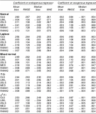
Tables 1 and 2 report mean bias and root mean squared er-ror (RMSE) for the estimators for each of the ve designs. The tables also report robust measures for bias and dispersion, the median bias, and median absolute error (MAE). As expected, the LIML and 2SLS estimators are superior to the other es-timators when the errors are normally distributed, and their performance deteriorates as the distribution of the errors be-comes more “thick tailed.” The estimators based on the ranks appear to be almost as efcient as the LIML and 2SLS even when the errors are normally distributed, and they are more ef-cient in essentially all of the other cases considered here. It
should be noted that except for theÂ2.1/, the errors in the de-signs other than the normal all have density at 0 greater than the normal. This will tend to make the asymptotic variance of the median-based estimators look relatively good. In an additional experiment (not reported in Tables 1 and 2), we found that if the errors are uniformly distributed (also normalized to have mean 0 and variance 1), then the MAE of the median-based estimator exceeds that of the 2SLS by almost 90%. In contrast, the MAE of the rank-based estimators exceeds that of the 2SLS by less than 10%.
A comparison of Tables 1 and 2 suggests that the relative per-mance of the estimators is not too sensitive to the distribution of the explanatory variables. We also increased the number of explanatory variables and instruments by 2; this did not change the relative performance of the estimators, although it did in-crease the computation time.
The asymptotic distributions presented in Section 2 and the Appendix allow one to do asymptotically valid inference, pro-vided that consistent estimators of the asymptotic variances of the estimators are available. The “numerical derivative” esti-mators of the asymptotic variances discussed in the Appendix require that the researcher choose a bandwidth. Because it is possible that the resulting inference is sensitive to the choice of bandwidth, it is interesting to investigate the small-sample properties of some simple test statistics constructed using some
34 Journal of Business & Economic Statistics, January 2004
Table 2. Small-Sample Performance of Alternative Estimators
Coefcient on endogenous regressor Coefcient on exogenous regressor
Mean Median Mean Median
bias RMSE bias MAE bias RMSE bias MAE
Normal
OLS :260 :267 :261 :261 :002 :084 ¡:001 :054 LIML ¡:004 :104 ¡:007 :071 :005 :103 :002 :069 2SLS :011 :108 :022 :067 :004 :098 :003 :068 MED ¡:041 :222 ¡:008 :101 :003 :139 ¡:005 :088 RANK1 ¡:011 :128 :003 :075 :005 :105 ¡:001 :069 RANK2 ¡:013 :131 :001 :075 :006 :109 :003 :072
Laplace
OLS :256 :264 :255 :255 :006 :090 :009 :063 LIML :000 :106 :001 :068 :003 :108 :008 :074 2SLS :015 :104 :024 :070 :005 :104 :009 :072 MED ¡:018 :129 ¡:002 :066 ¡:003 :104 :000 :064 RANK1 ¡:006 :100 :007 :062 :003 :093 :005 :061 RANK2 ¡:007 :105 :006 :064 :004 :094 :005 :063
Mixed normal
OLS :249 :262 :243 :243 :002 :090 :002 :058 LIML :001 :105 :009 :070 :003 :110 :002 :065 2SLS :006 :101 :016 :062 :003 :107 :001 :065 MED ¡:018 :103 ¡:006 :045 :002 :074 ¡:001 :047 RANK1 ¡:008 :069 ¡:005 :040 :001 :067 :001 :042 RANK2 ¡:009 :071 ¡:005 :042 :002 :068 ¡:001 :042
T.3/
OLS :244 :263 :230 :230 :000 :084 :002 :053 LIML :001 :140 :006 :067 ¡:001 :105 :000 :064 2SLS :010 :113 :014 :062 ¡:002 :099 :000 :063 MED ¡:020 :119 ¡:006 :062 ¡:005 :091 ¡:004 :060 RANK1 ¡:008 :086 ¡:001 :052 ¡:001 :077 ¡:003 :047 RANK2 ¡:008 :089 ¡:002 :055 ¡:001 :078 ¡:004 :051
Â2.1/
OLS :253 :266 :249 :249 ¡:004 :087 ¡:001 :059 LIML :000 :102 ¡:004 :069 ¡:003 :106 ¡:004 :068 2SLS :017 :108 :023 :069 ¡:003 :102 ¡:005 :067 MED ¡:061 1:593 ¡:015 :073 ¡:019 :427 ¡:005 :061 RANK1 :001 :051 :002 :026 ¡:002 :043 ¡:001 :023 RANK2 :001 :053 :002 :029 ¡:002 :045 ¡:002 :024
simple choices of bandwidth (and hence mimicking what re-searches might do in practice).
Table 3 presents the coverage probabilities of 80% con-dence intervals for each of the parameters in the designs dis-cussed earlier. These condence intervals are based on the bandwidth h D:1. When the bandwidth is small, the ma-trixb00Anb0was sometimes singular, (becauseb0is the numeri-cal derivative of a step function). When that happened,b00Anb0 was replaced byb00Anb0C10¡7I. Whereas choosinghD:1 is arbitrary, it seems of the proper order of magnitude, given the magnitudes of the explanatory variables. Table 3 also presents results forhD:05 andhD:2; the table suggests that for the chosen bandwidth, the numerical derivative estimates of the as-ymptotic standard errors for the two rank estimators perform pretty well (especially for the designs with symmetric errors), because thetstatistics based on those standard errors have ap-proximately the proper coverage probabilities. However, the es-timates of the standard errors for the median estimators do not perform as well; they seem to underestimate the standard er-rors and reject the null too often. One possible reason for this may be that the sample moment for the median estimator is less smooth than the ones for the rank estimators, because it in-volves a step function and only a single summation whereas the
double and triple summation for the two rank estimators tend to smooth things more. Therefore, the numerical derivative es-timates work less well for the median estimator.
Table 3. Coverage Probabilities 80%
hD:05 hD:1 hD:2
Normal
MED :66 :70 :70 :73 :70 :73 RANK1 :79 :78 :79 :77 :80 :78 RANK2 :79 :78 :79 :77 :80 :78
Laplace
MED :71 :75 :75 :78 :75 :78 RANK1 :79 :80 :80 :81 :82 :82 RANK2 :79 :80 :80 :81 :82 :82
Mixed normal
MED :72 :75 :77 :79 :77 :79 RANK1 :78 :76 :80 :78 :84 :81 RANK2 :78 :76 :80 :78 :84 :81
T.3/
MED :71 :72 :76 :76 :76 :76 RANK1 :76 :79 :76 :80 :80 :83 RANK2 :76 :79 :76 :80 :80 :83
Â2.1/
MED :64 :72 :70 :76 :70 :76 RANK1 :86 :87 :85 :87 :90 :91 RANK2 :86 :88 :87 :88 :90 :92
3.2 Empirical Examples
In this section we present two empirical examples. We use rst example to illustrate one strategy for calculating the es-timators discussed here, and demonstrate how to conduct tra-ditional inference based on the asymptotic distributions of the estimators. We use the second example to illustrate how one can use the moment conditions here to conduct inference in the spirit of Andersen and Rubin (1950). The second example also illustrates that using the techniques is computationally feasible even with very large datasets.
3.2.1 Example 1: Case and Deaton (1998). The rst ex-ample used to illustrate the estimators discussed here is the study by Case and Deaton (1998), which, among many other things, investigated the effect of the large cash transfers to the elderly on the food expenditures among African households in South Africa. They tested the hypothesis that “a rand is a rand”; that is, the pension income was spent in the same way as other income. More specically, they estimated the model with the food expenditures as the dependent variable and income ex-cluding pension and pension income, as the right-side vari-ables in addition to other explanatory varivari-ables controlling for household size and structures, regions, and other variables. The question then is whether the coefcients on those two income variables are the same. (See Case and Daeton 1998 for more details.)
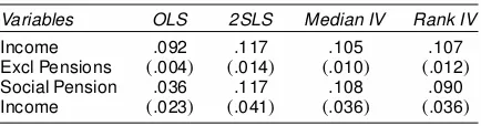
The possibility of measurement error and/or the endogeneity of the pension income in the foregoing regression model entails the IV estimation. Note that the pension income transfers were targeted specically at the age of the recipients, (i.e., only men over 65 and women over 60 were eligible), and the age was ex-ogenous; thus in one of many specications they used number of age-eligible females and number of age-eligible males as the instruments for the pension income receipts in the regression. In addition, a number of other variables (listed in Table 4) are used as instruments to deal with potential measurement errors in the two income variables. They found that the coefcients on the income excluding pension and pension income are both .117, as shown in Table 4. Both the median and the rank estimates are a little smaller in magnitude than 2SLS, and the difference between those two income variables are bigger, going from 0 to .003 for the median and to .02 for the rank estimators, al-though the differences still remain statistically insignicant.
In this example, both the estimates and the estimated stan-dard errors are very similar across the different estimators. This
Table 4. Estimates of Effect of Income on Food Expenditures
Variables OLS 2SLS Median IV Rank IV
Income :092 :117 :105 :107
Excl Pensions .:004/ .:014/ .:010/ .:012/
Social Pension :036 :117 :108 :090 Income .:023/ .:041/ .:036/ .:036/
NOTE: The specication is the same as in table V of Case and Deaton (1998). The sample size is 5,243. No weights are used in estimation. Other explanatory variables include household size; education of the head of the household, number of household members age 0–5, 6–15, 16–18, 19–21, and 22–24; age of house-hold head and its square; dummy for female headed househouse-hold; and province and metro dummies. Instruments are the number of women age 60 or older and the number of men age 65 or older, in addition to indicators that the head of house-hold is present; head is employed; head house-holds a regular wage job, a casual wage job, a job in agriculture, or a job in some other sector; head is paid monthly, forth-nightly, or weekly; and head is a dual job holder.
suggests that outliers might not be a big problem in this partic-ular application.
The standard errors for the median and rank IV estimators in Table 4 are calculated as discussed in the Appendix, where the choice of bandwidth is inspired by the Monte Carlo results discussed earlier. The exact formula for the bandwidth that we use is The factor of 100 makes it easier to make a comparison with the Monte Carlo experiments, which had nD100. We chose the bandwidth to be of the order of 1=4 the power of the sample size, because we wanted to undersmooth (relative to nonpara-metric regression or density estimation). The termmean[[ jx`j]
is meant to eliminate scale effects. We choosec as .8 for the median estimator and as .1 for the rank estimator. The motiva-tion for the latter is that the Monte Carlo study suggests that a bandwidth between .1 and .2 works well for the rank IV estima-tors for the designs considered there. WithcD:1, (13) would lead to a bandwidth of approximately .13 in the Monte Carlo experiment. The Monte Carlo study also suggests that a larger bandwidth should be used for the median IV estimator, which motivated the choicecD:8.
3.2.2 Example 2: Angrist, Imbens, and Krueger (1999). Because the estimators discussed in this article are nonlinear, it is potentially questionable whether they are useful in prac-tice for the very large sample sizes that are sometimes used for IV estimation. In this section we present one example where it is indeed possible to use the ideas presented here even when the sample size is very large. The application is taken from Angrist, Imbens, and Krueger (1999) and concerns estimation of the re-turns to schooling (see also Angrist and Krueger 1991). Angrist et al. (1999) used a variety of estimators to estimate the return to education based on 329,500 men born between 1930 and 1939. Here we use only the subset of 302,596 white men. Like Angrist et al. (1999), we consider a simple model in which the exoge-neous regressors are year effects and the instruments are year effects interacted with quarter of birth. The dependent variable is log weekly wage, and the (potentially) endogenous explana-tory variable is years of schooling.
Naively using (4), (7), (8), or (9) to estimate the returns to schooling involves 30 nondifferentiable moment conditions with 11 parameters. Computationally, this would be extremely time-consuming given the large sample size. We therefore pur-sue a slightly different strategy for estimating the coefcient on education. The model to be estimated is
lnwageiD° ¢EDUiCx0i¯C"i; (14) where xi are the exogenous explanatory variables, and "i is assumed to either satisfy quantile restrictions givenxi and the additional instruments,zi, or to be independent of.xi;zi/. The basic idea is to x° and then test whether the overidentifying restrictions are satised. The condence interval for° is then the set of° for which those restrictions are not rejected. This basic approach was proposed by Andersen and Rubin (1950), and the LIML estimator can be interpreted as minimizing such a test statistic. Later, we use the same idea to construct con-dence intervals for°. As is the case with the Andersen and
36 Journal of Business & Economic Statistics, January 2004
Rubin (1950) statistics, the test statistics are really joint tests of the value of ° and the overidentifying restrictions. Rejec-tions should therefore be interpreted as a rejection of the joint hypothesis that the instruments are valid and° equals the par-ticular value being considered.
Consider rst the case where one assumes that P."i·0j xi;zi/D®for some quantile,®. Then° measures the effect of an exogeneous change in education for somebody whose"i is at the®th quantile both before and after the exogenous change in education. In this case, (14) implies that
lnwagei¡° ¢EDUiDx0i¯C"i; P."i·0jxi/D®; (15) and for each candidate of°, ¯ can then be estimated by ap-plying standard quantile regression techniques to (15). One can then use the residuals, lnwagei¡° ¢EDUi¡x0i¯O, to test the additional moment conditions
E£¡¡.1¡®/¢ f"i·0g C®¢ f"i>0g
¢
zi
¤
D0: (16) This is asymptotically equivalent to performing a test of overi-dentifying restrictions on (3) for a xed° (see, e.g., Newey and McFadden 1994). Because it is by now quite easy to perform quantile regressions, this is much less time-consuming than it would be to test for overidentifying restrictions in (3) by rst calculating the efcient GMM estimator. Unfortunately, both approaches are complicated by the fact that the moment con-ditions are nondifferentiable, and one must therefore estimate the variance of the moments either by “smoothing” the moment conditions or by using the bootstrap. Because the variables inxi are all dummy variables in our application, the quantile regres-sion estimations can be performed by calculating cell quantiles. The computationsare therefore relatively easy, and it is feasible to use the bootstrap with a reasonably large number of replica-tions (we use 2,500). It should be noted that the asymptotics for the quantile regressions model assumes that"i(and henceyi) is continuously distributed. Unfortunately, the wage variable used here is not. This leads to “funny” results when the bootstrap is used to estimate the variance of the object in (16) when® is close to a point for which the distribution of"ihas point mass. The consequence of this is that the test statistics are quite un-smooth as function of°. In the results here, we have “cheated” by adding a little random noise to the log-wages. This makes the gures discussed later smoother than they would otherwise be.
Following the same strategy for moment conditions based on the ranks of the errors suggests rst estimating¯ (for xed°) by applying rank regression to
lnwagei¡° ¢EDUiDx0i¯C"i: (17) Unfortunately, the solution to this is not easy to calculate when the number of observations is large. We therefore use a slightly modied version of (6) to make inference about°.
Becausexiis composed of year dummies, independence be-tween"iandziin (17) implies that
cov[R.lnwagei¡° ¢EDUi/;zi]D0; (18) whereR.¢/is the rank of the argumentwithin each cohort. For xed°, we can therefore test the model by testing the 30 overi-dentifying restrictions that result from applying (18) to each of the 10 cohorts.
Figure 1. Andersen–Rubin Type Test Using ln(w) as a Dependent Variable ( AR; 25%; 50%; 75%; rank; critical value).
Figure 1 displays the test statistic associated with each value of° using the Andersen–Rubin (AR) statistic, the statistics as-sociated with the 25th, 50th, and 75th percentiles, as well as the one associated with the rank-statistic. In comparison, the point estimates reported by Angrist et al. (1999) are .089 for 2SLS, .093 for LIML, and .096 for the two so-called jacknife IV esti-mators. However, their sample differs from ours in that we use only white men. The graphs for the rank statistic and the AR statistic in Figure 1 are similar, suggesting that in this case the statistical model that assumes independence between"i andzi yields results similar to the model that assumes mean indepen-cence. For the quantiles however, it appears that for larger per-centiles, the statistic is minimized at smaller values of°. This suggests that the impact of education is larger at the lower end of the income distribution. This is the opposite of the effect found by Buchinsky (1994, table 1).
Figure 2 shows the results of the same calculations as in Fig-ure 1, but now with the level of wages as the dependentvariable. The main difference is that the level of the AR statistic is much
Figure 2. Andersen–Rubin Type Test Using w as a Dependent Vari-able ( AR; 25%; 50%; 75%; rank; critical value).
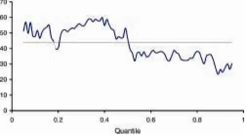
Figure 3. Test of Zero Coefcient on Education for Different Quantiles ( test statistic; critical value).
lower when wages rather than log-wages are used as the depen-dent variable. Because the more robust statistics based on the rank and the quantiles are similar in Figures 1 and 2, this might suggest that outliers play an important role for the AR statistic in Figure 2. However, unless° equals 0, the two models make different assumptions on the functional form of the relationship between wages and education. It is also possible that this could explain the difference in the AR.
Figures 1 and 2 suggest different returns to education at dif-ferent points in the wage distribution. We investigatethis further in Figure 3, which displays the test statistic for° D0 in (15) us-ing different values of®. Figure 3 suggests that the returns to education is positive for the lower half of the wage distribution, but that the signicance is questionable in the top half of the distribution.
4. CONCLUSION
This article has considered IV versions of the quantile and rank regression estimators. The proposed estimators provide al-ternatives to the conventional IV estimators. The advantage of these alternatives is that they are robust and hence much less sensitive to outliers. The disadvantage is that they are based on nonlinear moment conditions, and identication is there-fore assumed, rather than derived from primitive conditions. Except for this, it is easy to derive the asymptotic properties of the estimators and to estimate their asymptotic variances. We also conduct a small-scale Monte Carlo study to gauge the nite-sample performances of our estimators and the quality of the approximation to the nite-sample properties by asymptotic theories. We nd that the estimators perform very well in the de-signs that we consider, and that the asymptotic theory provides good approximations to the nite-sample properties of the es-timators. Finally, we apply our estimators to two empirical ex-amples. In the rst example, we estimate the effects of large cash transfers to the elderly on the food expenditures using the South African data; our estimators give slightly different results in comparison with the IV estimation, although the difference is within the sampling error. It is somewhat puzzling (and com-forting) that the estimators based on the ranks are so similar to those obtained by conventional IV. This might be due to the fact that the data we use here have already been “cleaned” up beforehand and so outliers are not a major problem. But our
estimators should provide more reliable results when the data are badly contaminated. In the second example, we revisit the Angrist et al. (1999) study of returns to education. This example demonstrates that it is feasible to implement the ideas discussed in this article, even with very large datasets. In this example, we use these ideas to study the differences in the returns to educa-tion across the distribueduca-tion of wages.
One possible extension of this article would consider exact (in nite samples) inference based on the moment conditions of this article. At the true parameter value, it is straightforward (but quite cumbersome) to derive the exact distributions of (4), and (7)–(9) (conditional on fzig). This in turn could be used to construct test statistics and condence intervals for the pa-rameters of the model. Such a procedure would be valid even if the implicit identication assumption of this article was not satised, although, of course, the resulting condence interval would not necessarily be a correct condence interval for the identication region.
ACKNOWLEDGMENTS
The authors thank Anne Case and David Jaeger for help-ing obtain the data used in this article and to Alan Kruger, the referees, and the editors for valuable comments. The au-thors gratefully acknowledge nancial support from the Na-tional Science Foundation (SES-0111342, SBR-9709598, and SES-0111799), the Wilson Society, the Danish National Re-search Foundation, and the Econometric ReRe-search Program at Princeton University. Part of this research was conducted when Bo Honoré visited the University of Copenhagen in the Fall of 1997. Their hospitality is also gratefully acknowledged.
APPENDIX: DETAILS ON IMPLEMENTATION A.1 Some Computational Issues
For the Monte Carlo study, we apply a sequence of mini-mizing methods to minimize the objective functions dening the estimators. The two main minimizing methods used are the downhill simplex method (amoeba) and Powell’s method, as described by Press, Flannery, Teukolsky, and Vetterling (1986). We rst scale the explanatory variables so that the changes in the parameters in the subsequent minimization are of compa-rable magnitudes. We then implement the minimization in four steps:
1. We start with downhill simplex method. That method requireskC1 starting values, where k is the number of pa-rameters. We use the OLS estimate as one starting point; the remaining starting points are obtained fromkone–dimensional grid searches on lines through the OLS estimate.
2. We minimize using Powell’s method, starting at the min-imum found in step 1.
3. We restart the downhill simplex method 10 times. In each minimization, we use the previous minimizer as one starting point and obtain the otherkstarting points by 10 different ad hoc deviations from that point. If that further reduces the func-tion value, then we repeat the sequence of 10 downhill simplex minimizations. If the latest sequence of 10 downhill simplex minimizations does not improve the function value, but the to-tal sequence of downhill simplex minimizations does, then we go back to step 2. Otherwise, we proceed to step 4.
38 Journal of Business & Economic Statistics, January 2004
4. We perform grid search for each parameter (xing the others at the current minimizer). If this improves the function value, then we go back to step 1. Otherwise, we perform a new set of grid searches using a different grid. If this improves the function value then we go back to step 1. Otherwise, we stop.
The estimates for the empirical examples were calculated in a similar way, except that we started from the result of a grid search on the line connecting the OLS and the 2SLS estimates.
A.2 The Variance of the Rank-Based Estimators
As mentioned in Section 2, it is relatively straightforward to derive the asymptotic properties for the rank-based estima-tors from the results of, for example, Sherman (1993, 1994) or Hono´re and Powell (1994). Specically, the estimator based on (7) is asymptotically equivalent to the estimator based on
1
which is a second-orderV statistic. The reason for this is that because the difference between those two sample moments is
1
2nzDOp.n¡
1/if E.z/ <1, the difference between the two
corresponding estimators is alsoOp.n¡1/. (See Robinson 1988 for the general results for differentiable moment functions and Andrews 1997 for the nondifferentiable case.)
The asymptotic distribution of the estimator dened by min-imization of the norm of (7) can then be found by a simple application of the results of Honoré and Powell (1994). Let si´.yi;xi;zi/and dene
andAis (the probability limit of) the weighting matrix. It is equally simple to derive the asymptotic distribution for the other rank IV estimators dened by (8) and (9). For exam-ple, the estimator based on
cov¡R."/;R.z/¢D0 can be implemented by minimizing the norm of
1
andAis (the probability limit of) the weighting matrix.
A.3 Consistent Estimator of the Covariance Matrix
The asymptotic distributions in (10)–(12) all depend on un-known matrices. Of these,E[ziz0i] in (10) and the twoVmatrices in.11/and (12) can be estimated by sample averages.
The matrix E[f"jx.0/x0izi] in (10) and the two Hmatrices in (11) and (12) are more complicated, because they are dened in terms of densities. To estimate these, we could either make distributional assumptions or use some nonparametric estima-tion technique. However, as pointed out by Pakes and Pollard (1989) and used by Honoré and Powell (1994), the derivation of the asymptotic normality implicitly implies that they can also be estimated by a “numerical derivative.”Specically, write (4), (7), and (8) asGn.b/. ThenE[f"jx.0/x0izi] in.10/and the two Hmatrices in.11/and.12/are then the derivatives ofE[Gn.b/] evaluated at¯. This suggests estimating thelth column of those matrices by identity matrix. The estimateb0 is consistent as long asan sat-ises
anDop.1/ and .pnan/¡1DOp.1/ asn! 1: One example may beanDn¡´for´ <1=2.
[Received November 2001. Revised April 2003.]
REFERENCES
Abadie, A. (1995), “Changes in Spanish Labor Income Structure During the 1980’s: A Quantile Regression Approach,” Working Paper 9521, CEMFI, Madrid, Spain.
Abadie, A., Angrist, J., and Imbens, G. (2002), “Instrumental Variables Estimates of the E ect of Subsidized Training on the Quantiles of Trainee Earnings,”Econometrica, 70, 91–117.
Abrevaya, J. (1999), “Leapfrog Estimation of a Fixed-Effects Model With Un-known Transformation of the Dependent Variable,”Journal of Econometrics, 93, 203–228.
(2000), “Rank Estimation of a Generalized Fixed-Effects Regression Model,”Journal of Econometrics, 95, 1–23.
Adichie, J. N. (1967), “Estimates of Regression Coefcients Based on Ranks,”
Annals of Mathematical Statistics, 38, 894–904.
Amemiya, T. (1982), “Two Stage Least Absolute Deviations Estimators,”
Econometrica, 51, 689–711.
Andersen, T. W., and Rubin, H. (1950), “The Asymptotic Properties of Es-timates of the Parameters of a Single Equation in a Complete System of Stochastic Equations,”Annals of Mathematical Statistics, 21, 570–582. Andrews, D. (1997), “A Stopping Rule for the Computation of Generalized
Methods of Moments Estimators,”Econometrica, 65, 913–932.
Angrist, J., Imbens, G., and Krueger, A. (1999), “Jackknife Instrumental Vari-ables Estimation,”Journal of Applied Econometrics, 14, 57–67.
Angrist, J., and Krueger, A. (1991), “Does Compulsory School Attendance Affect Schooling and Earnings,” Quarterly Journal of Economics, 106, 979–1014.
Buchinsky, M. (1994), “Changes in the U.S. Wage Structure 1963–1987: Ap-plication of Quantile Regression,”Econometrica, 62, 405–458.
(1998), “Recent Advances in Quantile Regression Models—A Prac-tical Guideline for Empirical Research,”Journal of Human Resources, 33, 88–126.
Case, A., and Deaton, A. (1998), “Large Cash Transfers to the Elderly in South Africa,”Economic Journal, 108, 1330–1361.
Cavanagh, C., and Sherman, R. (1998), “Rank Estimators for Monotonic Index Models,”Journal of Econometrics, 84, 351–381.
Durbin, J. (1954), “Errors in Variables,” International Statistical Review, 23–32.
Han, A. K. (1987), “Non-Parametric Analysis of a Generalized Regression Model: The Maximum Rank Correlation Estimator,”Journal of Economet-rics, 35, 303–316.
Hong, H., and Tamer, E. (2003), “Inference in Censored Models With Endoge-nous Regressors,”Econometrica, 71, 905–932.
Honoré, B., and Powell, J. (1994), “ Pairwise Difference Estimators of Cen-sored and Truncated Regression Models,” Journal of Econometrics, 64, 241–278.
Jaeckel, L. A. (1972), “Estimating Regression Coefcients by Minimizing the Dispersion of the Residuals,”Annals of Mathematical Statistics, 43, 1449–1458.
Jurecková, J. (1971), “Nonparametric Estimate of Regression Coefcients,”Ï An-nals of Mathematical Statistics, 42, 1328–1338.
Koenker, R., and Bassett, G. (1978), “Regression Quantiles,”Econometrica, 46, 33–50.
Newey, W., and McFadden, D. (1994), “Large Sample Estimation and Hy-pothesis Testing,” inHandbook of Econometrics, Vol. 4, eds. R. Engle and D. McFadden. New York, NY: Elsevier, pp. 2111–2245.
Pakes, A., and Pollard, D. (1989), “Simulation and the Asymptotics of Opti-mization Estimators,”Econometrica, 57, 1027–1057.
Press, W. H., Flannery, B. P., Teukolsky, S. A., and Vetterling, W. T. (1986),
Numerical Recipes: The Art of Scientic Computing, Cambridge, U.K.: Cam-bridge University Press.
Robinson, P. (1988), “The Stochastic Difference Between Econometric Statis-tics,”Econometrica, 56, 531–548.
Sakata, S. (2001), “Instrumental Variables Estimator Based on Mean Absolute Deviation,” Working paper, University of Michigan,
Sering, R. (1980),Approximation Theorems of Mathematical Statistics, New York: Wiley.
Sherman, R. (1993), “The Limiting Distribution of Maximum Rank Correlation Estimator,”Econometrica, 61, 123–137.
(1994), “U-Processes in the Analysis of a Generalized Semiparametric Regression Estimator,”Econometric Theory, 10, 372–395.
Silverman, B. (1986),Density Estimation for Statistical and Data Analysis, New York: Chapman & Hall.