07350015%2E2014%2E922471

(1)

Full Terms & Conditions of access and use can be found at

http://www.tandfonline.com/action/journalInformation?journalCode=ubes20

Download by: [Universitas Maritim Raja Ali Haji] Date: 11 January 2016, At: 19:17

Journal of Business & Economic Statistics

ISSN: 0735-0015 (Print) 1537-2707 (Online) Journal homepage: http://www.tandfonline.com/loi/ubes20

Empirical Analysis of Affine Versus Nonaffine

Variance Specifications in Jump-Diffusion Models

for Equity Indices

Katja Ignatieva, Paulo Rodrigues & Norman Seeger

To cite this article: Katja Ignatieva, Paulo Rodrigues & Norman Seeger (2015) Empirical Analysis of Affine Versus Nonaffine Variance Specifications in Jump-Diffusion Models for Equity Indices, Journal of Business & Economic Statistics, 33:1, 68-75, DOI:

10.1080/07350015.2014.922471

To link to this article: http://dx.doi.org/10.1080/07350015.2014.922471

Accepted author version posted online: 15 Sep 2014.

Submit your article to this journal

Article views: 161

View related articles

(2)

Empirical Analysis of Affine Versus Nonaffine

Variance Specifications in Jump-Diffusion

Models for Equity Indices

Katja I

GNATIEVA

School of Risk and Actuarial Studies, Australian School of Business, University of New South Wales Sydney, Sydney NSW 2052, Australia(k.ignatieva@unsw.edu.au)

Paulo R

ODRIGUES

Finance Department, Maastricht University, 6211 LM Maastricht, Netherlands (p.rodrigues@maastrichtuniversity.nl)

Norman S

EEGER

Finance Department, VU University Amsterdam, 1084 HV Amsterdam, Netherlands(n.j.seeger@vu.nl)

This article investigates several crucial issues that arise when modeling equity returns with stochastic variance. (i) Does the model need to include jumps even when using a nonaffine variance specification? We find that jump models clearly outperform pure stochastic volatility models. (ii) How do affine variance specifications perform when compared to nonaffine models in a jump diffusion setup? We find that nonaffine specifications outperform affine models, even after including jumps.

Keywords: Bayesian inference; Deviance information criteria; Markov chain Monte Carlo; Stochastic volatility.

1. INTRODUCTION

The objective of this article is to investigate and compare two strands of the literature concerned with modeling equity returns. On the one hand, Jones (2003b), Bakshi, Ju, and Ou-Yang (2006), Christoffersen, Jacobs, and Mimouni (2010), and Chourdakis and Dotsis (2011) proposed drift and diffusion spec-ifications for the variance process that result in a nonaffine model framework. However, in these papers, neither jumps in returns nor jumps in variance are considered important model com-ponents. In contrast, Eraker, Johannes, and Polson (2003) and Broadie, Chernov, and Johannes (2007) included jump compo-nents in the return and variance process, but preserved the drift and the diffusion term of the variance process in such a way that their models continue to be affine models.

The difference between these specifications is important. Both approaches employ a stochastic volatility term, but use dif-ferent procedures to model sudden large movements in the price and variance process. The nonaffine specification introduces nonlinearities into the drift and diffusion term of the variance process. This provides more flexibility when attempting to cap-ture large sudden movements in returns and variance, compared with the linear structure of an affine specification. The second approach generates large movements in returns and variance by staying within an affine framework and assuming a discontinu-ity in the price and, possibly, the variance process modeled via a jump component. The advantage of staying within the affine model class, analyzed in Duffie, Pan, and Singleton (2000), is that it allows for quasi-closed-form solutions for European op-tion prices, portfolio rules, and the computaop-tion of transiop-tion densities, all of which are advantageous for practical imple-mentation. Furthermore, the mathematical properties of these

models are well understood. The nonaffine models lack these benefits.

Our empirical analysis is designed to answer the question of whether we can disregard a jump component when modeling the variance process in a nonaffine way? Empirical studies, for ex-ample, by Jones (2003b), Bakshi, Ju, and Ou-Yang (2006), and Chourdakis and Dotsis (2011) propose nonaffine models that ig-nore jumps, and model extreme return and variance movements by means of nonlinear structures in the drift and diffusion com-ponent of the variance process. However, there is a strand of lit-erature in which a nonparametric model setup is used to analyze whether jumps in returns and jumps in variance are important model components; see, for example, Lee and Mykland (2008), A¨ıt-Sahalia and Jacod (2010), Barndorff-Nielsen and Shephard (2006), Corsi, Pirino, and Ren`o (2010), and Dumitru and Urga (2012). These studies find that jumps are indeed an important model component. Motivated by these results, we analyze, in a parametric model setup, whether nonlinearities and jumps are in fact substitutes for each other or whether including jumps can improve model performance even beyond the introduction of nonlinearities. Our findings clearly show that jumps do indeed play an important role in modeling the return process of a ma-jor equity index like the S&P 500 even after leaving the affine model class. Specifically, we find that even the worst performing jump model outperforms every pure stochastic volatility model considered.

68

(3)

Ignatieva, Rodrigues, and Seeger: Empirical Analysis of Affine Versus Nonaffine Variance Specifications 69

A second, subordinate question analyzed is whether a non-affine specification outperforms an non-affine specification within a jump diffusion setting. It has been shown in the literature, for example, by Jones (2003b), Bakshi, Ju, and Ou-Yang (2006), Christoffersen, Jacobs, and Mimouni (2010), and Chourdakis and Dotsis (2011) that this is indeed the case in a pure stochas-tic volatility setting. This question relates to the principle of keeping a model specification as simple as possible. The higher computational costs of using a nonaffine model instead of the more familiar affine specification can be justified only if the nonaffine specification results in significantly better model per-formance. With regard to this question, we find that nonaffine specifications do perform considerably better than affine setups even after including a jump term.

2. MODEL DESCRIPTION

We assume that the logarithm of the index priceYt=ln(St)

and the varianceVt solve the following system of stochastic

differential equations:

wheredWtyanddWtvdenote Brownian increments with

correla-tionE(dWtydWtv)=ρ dt, withρmodeling the so-called

lever-age effect. The termµcaptures the expected return,Ntdenotes a

Poisson process with constant intensityλ. The Poisson process enters both the return and variance equation, thus generating simultaneous jumps. The parametersξy andξvdenote, respec-tively, jump sizes in returns and variance. We assume that the jump sizes in variance and returns are correlated. The jump size in variance follow an exponential distribution with expectation

µv, that is,ξtv∼exp(µv), and the jump sizes in returns follow a

conditional normal distribution with mean given byµy+ρjξtv

and variance given byσ2

y, that is,ξ This model setup results in a general and flexible framework that subsumes a large number of modeling approaches proposed and tested independently in the related literature. By restricting the full model setup to various special cases, we can compare the performance of the different approaches to modeling the evolution of equity dynamics.

The return process in Equation (1) is based on Bates (1996), in which a combination of a stochastic volatility and jumps in returns model is used to analyze exchange rate processes. That is, for modeling jumps we employ a jump model with stochas-tic jump sizes and constant jump intensity, a framework that is frequently used in the literature; see, for example, Eraker, Johannes, and Polson (2003), Broadie, Chernov, and Johannes (2007), Durham (2013), or Ferriani and Pastorello (2012). The variance process in Equation (2) nests several specifications used in the literature. In the full model, the drift component of

the variance process follows a polynomial specification (POLY) that is applied in, for example, Conley et al. (1997) and A¨ıt-Sahalia (1996) to analyze short rate models and in Chourdakis and Dotsis (2011) to analyze stochastic volatility models with-out a jump component in the context of equity returns. The diffusion part of the variance is modeled as a constant elasticity of variance (CEV) specification where the exponent parame-terb of the variance is undetermined and is estimated freely. Jones (2003b) used this specification to analyze equity indices. Modeling jumps in variance follows the specification given in Eraker, Johannes, and Polson (2003).

To answer our research questions, we compare the full unre-stricted model described in Equation (1) and Equation (2) with several restricted specifications. We differentiate three main model classes in terms of how jump components are treated. Models with jumps in returns and variance are assigned to the stochastic volatility with correlated jumps (SVCJ) model class. Models that keep jumps in returns but remove them from the variance process are in the SVJ model class. Finally, models that switch off jumps in both the return and the variance process are in the pure stochastic volatility (SV) model class. Within each model class, we further classify models according to how the drift and diffusion components of the variance process are specified. Restricting the POLY drift component in Equation (2) by settingα1 andα3equal to zero, we obtain an affine lin-ear drift specification (ALIN). For the diffusion component in Equation2, Christoffersen, Jacobs, and Mimouni (2010) sug-gested specifications in which the CEV exponent parameterb

is restricted to 0.5, 1, or 1.5, termed SQR, ONE, or 3/2, respec-tively. Combinations of the aforementioned restrictions make up many well-known model specifications. For example, not considering jumps and combining an ALIN drift specification with a square root diffusion specification, SQR, results in the famous SV model of Heston (1993).

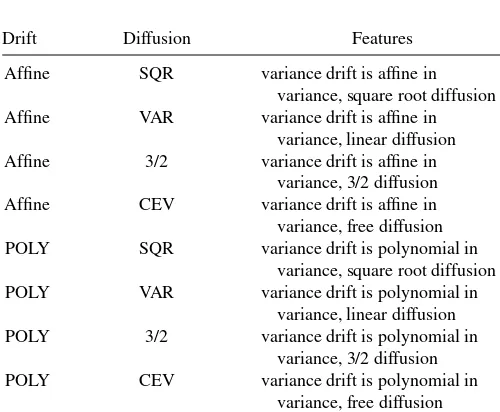
Having three model classes (SV, SVJ, SVCJ), two variance drift specifications (POLY, ALIN), and four variance diffusion specifications (CEV, SQR, ONE, 3/2) results in a total of 24 models to analyze, which are listed in Table 1. However, to avoid overloading the article with too many results, we only present results in detail that are useful for answering our research questions. The decision on which results to present is based on model performance, and statistical and economic reasoning. The complete results are available from the authors on request.

3. EMPIRICAL IMPLEMENTATION

3.1 Discretization

To estimate the model, we use an Euler discretization scheme and set the interval at ₌1, which corresponds to one day. DenotingRt =Yt−Yt−1as the log-return of the asset, we can

write the discretized version of the system of equations given in (1) and (2) as

(4)

Table 1. Overview of models

Drift Diffusion Features

Affine SQR variance drift is affine in variance, square root diffusion Affine VAR variance drift is affine in

variance, linear diffusion Affine 3/2 variance drift is affine in

variance, 3/2 diffusion Affine CEV variance drift is affine in variance, free diffusion POLY SQR variance drift is polynomial in

variance, square root diffusion POLY VAR variance drift is polynomial in

variance, linear diffusion POLY 3/2 variance drift is polynomial in

variance, 3/2 diffusion POLY CEV variance drift is polynomial in

variance, free diffusion

NOTE: This table shows the different specifications of the drift and diffusion terms for the dynamics of the stochastic variance. For each model class SV, SVJ, and SVCJ, we estimate every specification given in the table.

where shocks to returns and volatility, εy_t ₌W_ty₋W_ty₋₁ and

εv

t =Wtv−1−W

v

t−1, follow a bivariate normal distribution with

zero expectation, unit variance, and correlationρ. In the Euler discretization scheme, we assume at most one jump per day be-cause, given the observation frequency, we cannot distinguish between “more jumps” and “bigger jumps.” That is, the indi-cator Jt is set equal to one in the event a jump occurs and

equal to zero in the case of no jump. Note that the jump in-dicatorJt in the return equation is identical to the indicator in

the variance equation since jumps occur simultaneously. The jump sizes retain the distributional assumptions described in Section2.

The assumption of at most one jump per day could lead to some discretization bias when estimating jump parameters. However, the following example demonstrates that since jumps are rare events, discretization bias is typically very small. Using

P(Nt−Nt−1=j)= exp{−λ}λ

j

j! and assuming the jump

inten-sity to beλ₌0.1, the probability of observing more than one jump per day is 0.0047. Note that our estimation results indicate estimates forλmuch smaller than 0.1.

For technical details concerning the discretization schemes and the existence of stationary distributions of the models, as well as simulation results, the reader is referred to Jones (2003b), Eraker, Johannes, and Polson (2003), Jones (2003a), A¨ıt-Sahalia (1996), and Conley et al. (1997).

3.2 Estimation

We employ a Bayesian estimation and model testing strategy for our empirical investigation. These procedures were first used in the context of estimating continuous time models for equity returns by Jacquier, Polson, and Rossi (1994) and Jacquier, Pol-son, and Rossi (2004). Since then, these methods have been suc-cessfully employed in many empirical studies. In the following section, we provide an overview of the sampling algorithm for

a SVCJ model, since this is the most complex setup used in our analysis. Estimation of the restricted models accordingly fol-lows. For a general introduction to MCMC methods, the reader is referred to Casella and George (1992), Chib and Greenberg (1995), and Johannes and Polson (2009).

Bayes’ theorem implies that the posterior distribution of the parameters and the latent states is proportional to the likeli-hood times the prior distribution. Using the Euler discretized version of the models, it follows that the posterior distribution is proportional to

ter vector of the joint distribution of returns and variance and

_{denotes the full parameter vector comprising all}

parame-ters of the model. We assume independent conjugate priors for the parameters, so that the prior for the full parameter vector

p(_{) can be decomposed into the product of these priors. The}

prior parameters are set in accordance with Eraker, Johannes, and Polson (2003), Jacquier, Polson, and Rossi (2004), and Li, Wells, and Yu (2008). In our application, we use a sampler that draws one parameter and latent state at a time. Therefore, it is convenient to decompose the bivariate distribution of return and variance in Equation(4)into the product of a conditional and a marginal distribution. Given the Euler discretization, the bivari-ate distribution is normal with mean vectorm and covariance

matrixsgiven by s, further decomposition of the bivariate distribution into the

product of a conditional distribution times a marginal distribu-tion is straightforward.

To derive the complete conditionals for a parameter, we sim-ply remove all multiplicative factors from the posterior given in (4) that do not contain the parameter itself. Following this approach, the complete conditional for the parameterµis pro-portional to

where the conditional distribution is normal with parameters

µR|V =µ+ξ

distributed, and rearranging terms, we derive the following

(5)

whereµcan be interpreted as a regression coefficient. As such, we use its full conditional distribution in an MCMC step to draw

µ.

The complete conditional forα0is proportional to

T

where the conditional distribution is normal with parameters given by

Using the conditional normal property and by rearranging terms we can derive the following regression model:

Vt−Vt−1−b(Vt−1)+ξtvJt−ρσvVtb−−10.5(Rt−µ−ξ

Again, by using the regression model in Equation (6) and a stan-dard normally distributed prior, we can derive the parameter of the complete conditional distribution forα0. Estimation of the remainingαparameters consists simply of varying the regres-sion setup of Equation (6), where we assume identical prior distributions for allαparameters.

To draw the parametersρandσv, we follow Jacquier, Polson,

and Rossi (2004) and define φ_≡ρσv and ω2≡σv2(1−ρ

2_).

Drawingφandω2_{amounts to using a regression setup given by} Vt−Vt−1−a(Vt−1)−ξtvJt prior distributions, and IG denotes an inverse Gamma distri-bution.

The complete conditional distribution for the jump parameters

µy,ρJ, andσyis given by

eters, the following regression setup is used

ξty =µy+ρJξtv+σyε.

For the parameterµv, the complete conditional takes the form T

t=1

p(ξ_tv_|µv)p(µv),

where we take IG (10,1/10) as the prior distribution for µv.

Standard results given in, for example, Bernardo and Smith (1995) show that the resulting complete conditional forµv is

inverse Gamma.

For the parameterλ, we assume a Beta distribution (B(2,40)) as prior. The complete conditional given by

T

t=1

p(Jt|λ)p(λ) (7)

is a combination of a binomial distribution and a Beta distri-bution. Standard results given in, for example, Bernardo and Smith (1995) show that the complete conditional follows a Beta distribution.

For the parameter b, we discretize the space into bins with equal prior probability, that is, we assume b₌ {0.5,0.502,0.504, . . . ,2.5}. The complete conditional forb fol-lows a multinomial distribution where the probability for each bin is proportional to

where the superscriptiindicates that expression (8) is evaluated at the value thatbhas for the respective bini. We note that in this particular case, the prior probabilities will drop out of the calculation of the complete conditional, since they are identical for all bins.

The state variables, Jt, ξ y

t, ξtv, and Vt are drawn

sequen-tially for each t. The jump indicator Jt follows a binomial

distribution with complete conditional probabilities propor-tional to λp(Rt, Vt|Vt−1, ξtv, ξ

For the jump sizes in returns, the complete conditional forξty

is proportional to

which is normally distributed with parameters that are easy, albeit tedious, to compute. For the case of Jt =0, we

sim-ply draw from the prior distribution, since the data provide no information.

The derivation of the complete conditional distribution for the jump sizes in variance follows similar lines. The complete conditional is given by

which results in a truncated normal distribution with parameters that are straightforward to compute. In the case ofJt =0, we

draw from the prior, since the data provide no information. ForVt, the complete conditional is given by

p(Rt+1, Vt+1|Vt, Jt−1, ξtv+1, ξ

y

t+1,RV)

×p(Vt|Rt, Vt−1, ξtv, Jt,R,V),

which does not resemble any known statistical distribution. We, therefore, use the Metropolis–Hastings step to draw variances

(6)

from their complete conditional distributions. We follow Chib and Greenberg (1995) and Jones (2003b) in using the recogniz-able part of the complete conditional as the proposal density, that is, we drawVt fromp(Vt|Rt, Vt−1, ξtv, Jt,R,V). The

ac-ceptance probability for the draw is given by

min

p(Rt+1, Vt+1|V (g)

t , Jt−1, ξtv+1, ξ

y

t+1,RV)

p(Rt+1, Vt+1|V (g−1)

t , Jt−1, ξtv+1, ξ

y

t+1,RV)

,1

,

whereVt(g)indicates the proposed value andV

(g−1)

t denotes the

current draw. That is, by usingVt−1andRt to obtain candidate

draws, we use information in the data to increase the acceptance probability. Our acceptance rates are around 65%, which is nearly identical to the rates reported in Jones (2003b).

3.3 Model Comparison

Comparing and then ranking the models in our model setup is not easily accomplished. In theory, the most convincing statis-tics for model comparison are Bayes’ factors. But although they are theoretically appealing, these statistics are difficult to compute for very high-dimensional problems like those under consideration. In certain cases, for example comparing jump models to models without jumps, Eraker, Johannes, and Polson (2003) showed how to use the structure of these nested models to compute the Bayes’ factors. For these cases, we follow their pro-cedure and so can use the Bayes’ factors for model comparison. To compare nonnested models, we rely on the deviance informa-tion criterion (DIC) derived in Spiegelhalter et al. (2002). This information criterion uses the same structure as any information criterion, namely, it penalizes model complexity and rewards model fit. The only difference is that the DIC accounts for the hierarchical structure of our models in determining model com-plexity. DIC is employed to compare stochastic variance models for equity index returns by, for example, Berg, Meyer, and Yu (2004).

3.4 Model Implementation

Implementation of the MCMC algorithm is carried out in C++ using random number generators of the GNU Scientific Library. Since the MCMC method is by construction a sequen-tial algorithm (each draw depends on the preceding draw), there is limited potential to decrease computational time by paral-lelizing the algorithm. However, the dependence structure of the variances can be used to draw variances in blocks of two, as is done in Jones (2003b), which at least offers the possibil-ity of some performance gain by parallelization. Convergence of model parameters relies heavily on the model specification to be estimated. For a SV-ALIN-SQR model, convergence can be obtained relatively quickly by drawing 50,000 times with a burn-in period of 10,000 draws, whereas for a more complex model such as SVCJ-POLY-CEV, convergence is obtained after 300,000 draws with a burn-in period of 100,000. Note that calcu-lating stable values for the DIC statistics and, therefore, a stable ranking of the models in terms of DIC is more sensitive to the number of MCMC draws than is the calculation of the parame-ters. Thus, to ensure convergence of all models in parameters and to obtain a stable ranking in terms of DIC, we base our

estima-tion results on 2 million draws with a burn-in period of 600,000 draws. Again, the run time for a full model estimation is strongly dependent on the model specification to be estimated. We per-form our calculations on a large computer cluster equipped with Intel Xeon L5520 2.26 GHz processors. Our setup of 2 million MCMC draws results in an estimation time of about 4.5 hr for the SV-ALIN-SQR, 5.2 hr for the SVCJ-POLY-3/2 model with fixedb, and about 28 hr for the SVCJ-POLY-CEV model with estimatedbparameter.

4. RESULTS

4.1 Data and Parameter Estimates

We analyze model performance using a time series of daily log returns of the S&P 500 index. Data of S&P 500 simple returns are taken from CRSP (crsp variable name “sprtrn”), which are calculated close-to-close. Simple returns are con-verted to log returns and the dataset covers the period from January 1980 to December 2010. The mean return for the time period is about 8% p.a. with a volatility of about 18% p.a. The S&P 500 index had negative skewness of about−1.21 and a kurtosis of about 31 indicating fat tails in the period under analysis, where both numbers refer to a daily period. To check whether our results are driven by the recent financial crisis we analyze model performance for the time period 1980–2007 and find no difference. These additional results are available upon request.

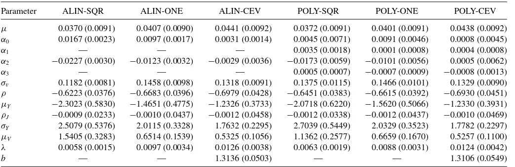
The parameter estimators for the models within the SVCJ class can be found in Table 2. We follow the convention of reporting our estimators in daily levels with the returns given in percentages, that is, we estimate the models and report the results with returns defined as 100·(lnSt−lnSt−1). Our

es-timated parameters for the models with a typical square root volatility specification are in line with what can be found in the literature; see, for example, Eraker, Johannes, and Polson (2003), Eraker (2004), and Christoffersen, Jacobs, and Mimouni (2010). We note that to compare the parameter estimates with other results in the literature, it is necessary to take into account the different ways to parameterize the mean reversion compo-nent in the variance process.

Given the focus of the analysis of our article, the estimates that warrant a more detailed discussion are jump parameters. We find that jumps are rare and have a large negative mean. For the SVCJ model we estimate a jump intensity ranging from 0.006 (SQR) to 0.013 (3/2), which translates into roughly 1.5 to 3.3 jumps per year. If we change the variance diffusion specification from SQR to ONE to CEV to 3/2 we see that the jump intensity increases for an increase in the exponent parameterb. For the mean jump sizes in returns, standard deviation of jump sizes in returns, and the mean jump size in variance, we find decreasing absolute values for increasing exponent parameterb. These values range from−2.7 (SQR) to−1.17 (3/2) for the mean return jump size, from 2.7 (SQR) to 1.7 (3/2) for the standard deviation in the return jumps, and from 1.5 (SQR) to 0.5 (3/2) for the jump size in variance. We note that the changes in parameter estimates when changing the exponent parameterboccur monotonically. Interestingly, we find almost no differences in the estimated jump parameters for the different drift specifications ALIN and

(7)

Table 2. Parameter estimators for the SVCJ model class

Parameter ALIN-SQR ALIN-ONE ALIN-CEV POLY-SQR POLY-ONE POLY-CEV

µ 0.0370 (0.0091) 0.0407 (0.0090) 0.0441 (0.0092) 0.0372 (0.0091) 0.0401 (0.0091) 0.0438 (0.0092) α0 0.0167 (0.0023) 0.0097 (0.0017) 0.0031 (0.0014) 0.0045 (0.0071) 0.0091 (0.0046) 0.0008 (0.0045)

α1 — — — 0.0035 (0.0018) 0.0001 (0.0008) 0.0004 (0.0008)

α2 −0.0227 (0.0030) −0.0123 (0.0032) −0.0029 (0.0036) −0.0173 (0.0059) −0.0101 (0.0056) 0.0005 (0.0062)

α3 — — — 0.0005 (0.0007) −0.0007 (0.0009) −0.0008 (0.0013)

σv 0.1182 (0.0081) 0.1458 (0.0098) 0.1318 (0.0091) 0.1375 (0.0115) 0.1466 (0.0101) 0.1329 (0.0090)

ρ ₋0.6223 (0.0376) ₋0.6683 (0.0396) ₋0.6979 (0.0428) ₋0.6451 (0.0383) ₋0.6615 (0.0392) ₋0.6930 (0.0451) µY −2.3023 (0.5830) −1.4651 (0.4775) −1.2326 (0.3733) −2.0718 (0.6220) −1.5620 (0.5066) −1.2330 (0.3931)

ρJ −0.0009 (0.0233) −0.0010 (0.0437) −0.0012 (0.0458) −0.0012 (0.0338) −0.0012 (0.0437) −0.0010 (0.0469)

σY 2.5079 (0.5376) 2.0115 (0.3328) 1.7632 (0.2295) 2.7039 (0.5449) 2.0329 (0.3523) 1.7782 (0.2297)

µV 1.5405 (0.3283) 0.6514 (0.1539) 0.5325 (0.1056) 1.1362 (0.2577) 0.6659 (0.1670) 0.5257 (0.1100)

λ 0.0058 (0.0015) 0.0097 (0.0034) 0.0126 (0.0038) 0.0063 (0.0019) 0.0088 (0.0031) 0.0124 (0.0042)

b — — 1.3136 (0.0503) — — 1.3106 (0.0549)

NOTE: This table shows the posterior means and standard deviations (in parentheses) for the ALIN and POLY drift specification in combination with a SQR, ONE, and CEV diffusion for the SVCJ model class. The details of the models are described in Section2. The underlying dataset consists of log-returns of the S&P index for the period from January 1980 until December 2010. Parameters are presented in daily percentage units.

POLY. These parameters are also in line with previous literature. For example, Eraker, Johannes, and Polson (2003) found a jump intensity of 0.0066 for the SVCJ-ALIN-SQR specification with a mean jump size in returns of−2.64 and a mean jump size in variance of 1.48. We observe the same effects for the SVJ model class.

However, some recent papers find jump components that do not fit these results. For example, Ferriani and Pastorello (2012) and Durham (2013) estimated very frequent jumps that have a slightly positive mean. Both papers use options, meaning that their information sets are different from ours. In particular, the article by Durham (2013) discusses extensively the origins of the differences between his estimation results concerning the jump component and those from the previous literature. One of the main reasons he identifies involves the prior distribution for the jump intensity used in the previous literature, which puts very low prior probability on frequent jumps, as is also true for our setup. We, therefore, analyze whether our prior puts a significant restriction on the posterior results. To do so, we change the prior distribution for the jump intensity from a Beta distribution to a multinomial distribution with discrete proba-bility mass for different parameter values. We decompose the prior parameter space for the jump intensity from 0.001 to 0.5 into intervals of 0.001, where each bin has equal prior proba-bility, thus assuming prior ignorance on the intensity level. In unreported results that are available on request, we find that the parameter estimates are virtually the same for both prior speci-fications, that is, Beta and Multinomial prior. This holds true for all jump models under consideration. Moreover, the posterior indicates zero probability for a jump intensity larger than 0.116, which shows that our choice of 0.5 as the upper limit for the discretized parameter space ofλimposes no restriction on the posterior. We, therefore, conclude that our posterior estimation results are driven by data rather than by restrictions on the prior distribution. Analyzing the exact reason for the different esti-mation results between our setup and the setup used in Ferriani and Pastorello (2012) and Durham (2013) is beyond the scope of this article, but presents an interesting possibility for future research.

4.2 Model Performance

A standard result from the literature analyzing affine mod-els is that jumps are important for explaining observed return dynamics. However, the studies analyzing nonaffine specifica-tions, such as Jones (2003b), Christoffersen, Jacobs, and Mi-mouni (2010), Bakshi, Ju, and Ou-Yang (2006), and Chourdakis and Dotsis (2011), treat the jump component as at most of sec-ondary importance, if it is even analyzed at all. There are several reasons for this quasi-disregard of the jump component in this branch of the literature. First, some authors focus on finding the best variance specification in a nonaffine setup, claiming that the results could be generalized to a setup with jumps. Second, to avoid the problem of overfitting, authors understandably wish to remain within the most parsimonious model specification, and thus focus on stochastic variance. We argue that the question of the best variance specification cannot be answered without simultaneously considering jumps, since the overall variance of a model is determined by the sum of a part driven by stochastic variance and a part driven by the jump component.

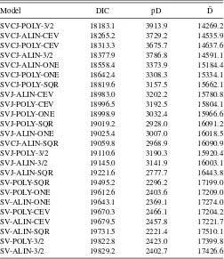
We answer the question of whether jumps are important by using our results from the DIC statistics and comparing Bayes’ factors.Table 3 clearly shows the dominance of jump models over pure SV specifications. All SV models are at the lower end of the table and thus 100% outperformed by the jump models. In other words, no matter how a SV model is specified, it can always be improved by including a jump component. In particular, we find that the best-performing pure SV specification (SV-POLY-SQR) does not necessarily produce the best-performing overall specification when a jump component is added. This result is strong evidence against the advisability of simply first choosing an optimal SV model and then adding a jump component.

The same result is seen from the Bayes’ factors shown inTable 4. Following the rule of thumb given in Kass and Raftery (1995) and interpreting a value greater than 6 as strong evidence in favor of the model listed first under the column heading, we see that the SV model is also rejected by the Bayes’ factors regardless of the specification of the variance process. Regarding the question of whether jumps can be disregarded when moving away from

(8)

Table 3. Rankings of models by DIC

Model DIC pD D¯

SVCJ-POLY-3/2 18183.1 3913.9 14269.2 SVCJ-ALIN-CEV 18265.2 3729.2 14535.9 SVCJ-POLY-CEV 18313.3 3675.7 14637.6 SVCJ-ALIN-3/2 18377.9 3786.8 14591.1 SVCJ-ALIN-ONE 18558.4 3373.9 15184.4 SVCJ-POLY-ONE 18642.4 3308.3 15334.1 SVCJ-POLY-SQR 18819.6 3157.5 15662.1 SVJ-ALIN-CEV 18983.0 3202.2 15780.8 SVJ-POLY-CEV 18996.5 3192.5 15804.1 SVJ-POLY-ONE 18998.9 3032.4 15966.6 SVJ-POLY-SQR 19019.2 2928.0 16091.2 SVJ-ALIN-ONE 19025.4 3007.0 16018.5 SVCJ-ALIN-SQR 19059.8 2968.9 16090.9 SVJ-POLY-3/2 19110.6 3190.3 15920.4 SVJ-ALIN-3/2 19145.0 3141.9 16003.1 SVJ-ALIN-SQR 19221.6 2777.7 16443.8 SV-POLY-SQR 19495.2 2296.2 17199.0 SV-POLY-ONE 19612.6 2403.6 17209.0 SV-ALIN-ONE 19643.1 2369.1 17274.0 SV-POLY-CEV 19670.3 2466.1 17204.2 SV-ALIN-CEV 19679.5 2457.8 17221.7 SV-ALIN-SQR 19731.5 2221.4 17510.1 SV-POLY-3/2 19822.8 2423.0 17399.8 SV-ALIN-3/2 19829.2 2402.7 17426.6

NOTE: This table shows the DIC rankings of the various models. The second and third columns show the values for model complexity and model fit, respectively. The details of the models are described in Section2. The underlying dataset consists of log-returns of the S&P index for the period from January 1980 until December 2010.

the affine model specification, we note that the Bayes’ factors even increase in the nonaffine specifications.

The results of the comparison between models with jumps in returns and models containing jumps in returns and variance are mixed. We see a clear outperformance of the SVCJ model class when looking at the DIC statistics, but this is not the case when the Bayes’ factors are used for model comparison. When using the Bayes’ factors as a means of comparison, we find strong evidence in favor of a SVJ model for two cases and weak evidence in favor of SVJ models in the remaining setups.

Table 4. Bayes’ factors

Drift & diffusion SVJ vs. SV SVCJ vs. SV SVCJ vs. SVJ

ALIN-SQR 31.1 8.0 ₋23.0

ALIN-ONE 46.6 43.5 ₋3.0

ALIN-3/2 49.4 45.8 ₋3.6

ALIN-CEV 48.9 46.1 ₋2.8

POLY-SQR 35.2 24.5 ₋10.6

POLY-ONE 46.5 41.2 ₋5.3

POLY-3/2 49.6 47.3 ₋2.3

POLY-CEV 48.6 46.3 ₋2.4

NOTE: This table shows the Bayes’ factors in a comparison of nested model specifications. The first two columns show the results for comparing the SVJ and the SVCJ models respectively with the SV model specification. The third column shows the results for comparing the SVJ and the SVCJ models. A positive value for the Bayes’ factor shows a preference for the model mentioned first in the column heading. The underlying dataset consists of log-returns of the S&P index for the period from January 1980 until December 2010.

In summary, we conclude that jumps are an important model component in explaining in-sample return dynamics regardless of whether the variance specification is affine or nonaffine.

It has been shown in the literature—see, for example, Jones (2003b), Bakshi, Ju, and Ou-Yang (2006), Christoffersen, Ja-cobs, and Mimouni (2010), and Chourdakis and Dotsis (2011)— that nonaffine models outperform their affine counterparts when looking at a pure SV specification. An interesting question that follows from the strong outperformance of jump diffusion mod-els when compared to pure SV modmod-els is whether nonaffine models still outperform their affine counterparts in a jump dif-fusion setup. This is an important question for a number of reasons. First, affine models are relatively well known with re-spect to their mathematical properties. Second, the economic implications of affine models in equilibrium models are also well known. Third, the technique of Duffie, Pan, and Single-ton (2000) can be used to calculate semiclosed-form solutions for prices of plain-vanilla options. None of the above men-tioned points are true of nonaffine models. The question of whether the better performance of the nonaffine models com-pared to the affine models justifies having to deal with the greater model complexity of the former therefore becomes of interest.

According toTable 3, all top-ranked models are of the non-affine type. The best non-affine specification, SVCJ-ALIN-SQR, ranks 12th. Since it is not possible to compute standard errors or distributions of DIC, we cannot judge what constitutes a significant difference in these statistics. We, therefore, use an ad-hoc approach to assessing model difference by looking at percentage differences relative to the best performing model in terms of the DIC statistics. The difference between the best and the worst model is about 9%, that is, we achieve a 9% im-provement in DIC when switching from the worst to the best model. The model improvement achieved by switching from the best affine model to the best overall model is about 4.8%. These numbers show that a substantial improvement in perfor-mance can be achieved by abandoning the affine model class. When comparing affine to nonaffine specifications within each model class, we find that the affine specification ranks last for the SVJ and SVCJ model class and third to last for the SV class.

5. CONCLUSION

We conduct a comprehensive empirical analysis of continuous-time models for equity index returns with the aim of investigating the properties of several widely used model classes, specifically affine and nonaffine stochastic variance specifications augmented by jump components. The results of our analysis lead us to the following conclusions. First, jump components are an important model component regardless of whether the setup is affine or nonaffine. Even the worst perform-ing jump model outperforms a pure SV specification in terms of DIC statistics. Furthermore, Bayes’ factors strongly favor jump models over pure diffusion models regardless of the variance setup. Second, nonaffine specifications perform considerably better than affine specifications even when jump components are included into the model.

(9)

ACKNOWLEDGMENTS

We thank Shakeeb Khan (Editor), Associate Editor, and two anonymous referees, for helpful guidance and constructive com-ments. For insightful discussions and suggestions, we thank Michael Johannes, Christian Schlag, Raman Uppal, Grigory Vilkov, Peter Schotman, Andr´e Lucas, Joao Cocco, Joachim Grammig, Pedro Santa-Clara, and seminar participants at the 2010 Meeting of the European Finance Association, 2010 FMA European Conference, 2010 World Congress of the Bachelier Finance Society, 2009 Annual Meeting of the German Finance Association (DGF), 2009 European Meeting of the Econometric Society, 2009 Far East and South Asia Meeting of the Econo-metric Society, 2009 International Conference on Computing in Economics and Finance, Econometric Society Australasian Meeting in 2009, and 2009 Meeting of the Swiss Society of Economics and Statistics. Any errors are, however, our re-sponsibility alone. A previous version of the article was cir-culated under the title of “Stochastic Volatility and Jumps: Exponentially Affine Yes or No? An Empirical Analysis of S&P500 Dynamics.” Financial support from the German Sci-ence Foundation is gratefully acknowledged. We thank SURF-sara (www.surfsara.nl) for support in using the Lisa Computer Cluster.

[Received September 2012. Revised April 2014.]

REFERENCES

A¨ıt-Sahalia, Y. (1996), “Testing Continuous-Time Models of the Spot Interest Rate,”Review of Financial Studies, 9, 385–426. [69,70]

A¨ıt-Sahalia, Y., and Jacod, J. (2010), “Is Brownian Motion Necessary to Model High-Frequency Data?”The Annals of Statistics, 38, 3093–3128. [68] Bakshi, G., Ju, N., and Ou-Yang, H. (2006), “Estimation of Continuous-Time

Models With an Application to Equity Volatility Dynamics,”Journal of Financial Economics, 82, 227–249. [68,73,74]

Barndorff-Nielsen, O. E., and Shephard, N. (2006), “Econometrics of Testing for Jumps in Financial Economics Using Bipower Variation,”Journal of Financial Econometrics, 4, 1–30. [68]

Bates, D. S. (1996), “Jumps and Stochastic Volatility: Exchange Rate Processes Implicit in Deutsche Mark Options,”Review of Financial Studies, 9, 69–107. [69]

Berg, A., Meyer, R., and Yu, J. (2004), “Deviance Information Criterion for Comparing Stochastic Volatility Models,”Journal of Business and Eco-nomic Statistics, 22, 107–120. [72]

Bernardo, J., and Smith, A. (1995),Bayesian Theory, New York: Wiley. [71] Broadie, M., Chernov, M., and Johannes, M. (2007), “Model Specification and

Rrisk Premia: Evidence From Futures Options,”The Journal of Finance, 62, 1453–1490. [68,69]

Casella, G., and George, E. I. (1992), “Explaining the Gibbs Sampler,”The American Statistician, 46, 167–174. [70]

Chib, S., and Greenberg, E. (1995), “Understanding the Metropolis-Hastings Algorithm,”The American Statistician, 49, 327–335. [70,72]

Chourdakis, K., and Dotsis, G. (2011), “Maximum Likelihood Estimation of Non-Affine Volatility Processes,”Journal of Empirical Finance, 18, 533– 545. [68,69,73,74]

Christoffersen, P., Jacobs, K., and Mimouni, K. (2010), “Volatility Dynamics for the S&P500: Evidence From Realized Volatility, Daily Returns, and Option Prices,”Review of Financial Studies, 23, 3141–3189. [68,69,72,73,74] Conley, T. G., Hansen, L. P., Luttmer, E. G. J., and Scheinkman, J. A. (1997),

“Short-Term Interest Rates as Subordinated Diffusions,”Review of Financial Studies, 10, 525–577. [69,70]

Corsi, F., Pirino, D., and Ren`o, R. (2010), “Threshold Bipower Variation and the Impact of Jumps on Volatility Forecasting,”Journal of Econometrics, 159, 276–288. [68]

Duffie, D., Pan, J., and Singleton, K. (2000), “Transform Analysis and Asset Pricing for Affine Jump-Diffusions,”Econometrica, 68, 1343–1376. [68,74] Dumitru, A.-M., and Urga, G. (2012), “Identifying Jumps in Financial Assets: A Comparison Between Nonparametric Jump Tests,”Journal of Business and Economic Statistics, 30, 242–255. [68]

Durham, G. (2013), “Risk-Neutral Modelling With Affine and Non-Affine Mod-els,”Journal of Financial Econometrics, 11, 650–681. [69,73]

Eraker, B. (2004), “Do Stock Prices and Volatility Jump? Reconciling Evidence From Spot and Option Prices,”The Journal of Finance, 59, 1367–1404. [72] Eraker, B., Johannes, M., and Polson, N. (2003), “The Impact of Jumps in Volatility and Returns,” The Journal of Finance, 58, 1269–1300. [68,69,70,72]

Ferriani, F., and Pastorello, S. (2012), “Estimating and Testing Non-Affine Option Pricing Models With a Large Unbalanced Panel of Options,”The Econometrics Journal, 15, 171–203. [69,73]

Heston, S. L. (1993), “A Closed-Form Solution for Options With Stochastic Volatility With Applications to Bond and Currency Options,”Review of Financial Studies, 6, 327–343. [69]

Jacquier, E., Polson, N. G., and Rossi, P. E. (1994), “Bayesian Analysis of Stochastic Volatility Models,”Journal of Business and Economic Statistics, 12, 371–389. [70]

——— (2004), “Bayesian Analysis of Stochastic Volatility Models With Fat-Tails and Correlated Errors,” Journal of Econometrics, 122, 185–212. [70,71]

Johannes, M., and Polson, N. (2009), “MCMC Methods for Continuous-Time Financial Econometrics,” inHandbook of Financial Econometrics(vol. 2), ed. Y. L. H. Ait-Sahalia, Oxford, UK: North Holland, pp. 1–72. [70] Jones, C. S. (2003a), “Nonlinear Mean Reversion in the Short-Term Interest

Rate,”Review of Financial Studies, 16, 793–843. [70]

——— (2003b), “The Dynamics of Stochastic Volatility: Evidence From Un-derlying and Options Markets,”Journal of Econometrics, 116, 181–224. [68,69,70,72,73,74]

Kass, R., and Raftery, A. (1995), “Bayes Factors,”Journal of the American Statistical Association, 90, 773–795. [73]

Lee, S. S., and Mykland, P. A. (2008), “Jumps in Financial Markets: A New Nonparametric Test and Jump Dynamics,”Review of Financial Studies, 21, 2535–2563. [68]

Li, H., Wells, M. T., and Yu, C. L. (2008), “A Bayesian Analysis of Return Dynamics With L´evy Jumps,”Review of Financial Studies, 21, 2345–2378. [70]

Spiegelhalter, D. J., Best, N. G., Carlin, B. P., and van der Linde, A. (2002), “Bayesian Measures of Model Complexity and Fit,”Journal of the Royal Statistical Society,Series B, 64, 583–639. [72]