Full Terms & Conditions of access and use can be found at
http://www.tandfonline.com/action/journalInformation?journalCode=ubes20
Download by: [Universitas Maritim Raja Ali Haji] Date: 12 January 2016, At: 00:14
Journal of Business & Economic Statistics
ISSN: 0735-0015 (Print) 1537-2707 (Online) Journal homepage: http://www.tandfonline.com/loi/ubes20
Missing Treatments
Francesca Molinari
To cite this article: Francesca Molinari (2010) Missing Treatments, Journal of Business & Economic Statistics, 28:1, 82-95, DOI: 10.1198/jbes.2009.07161
To link to this article: http://dx.doi.org/10.1198/jbes.2009.07161
Published online: 01 Jan 2012.
Submit your article to this journal
Article views: 193
View related articles
Missing Treatments
Francesca M
OLINARIDepartment of Economics, Cornell University, 492 Uris Hall, Ithaca, NY 14853-7601 (fm72@cornell.edu)
This article analyzes the problem of identifying a treatment effect with imperfect observability of the treatment received by the population. Imperfect observability may be due to item/survey nonresponse or to noncompliance with randomly assigned treatments. I derive sharp worst-case bounds that are a function of the available prior information on the distribution of missing treatments. Under the assumption of monotone treatment response, I show that prior information on the distribution of missing treatments is not necessary to get sharp informative bounds. I illustrate the results with an empirical analysis of drug use and employment using data from the National Longitudinal Survey of Youth.
KEY WORDS: Bounds; Missing data; Partial identification; Treatment effect.
1. INTRODUCTION
Part of the existing literature on program evaluation has ex-amined what can be inferred about a treatment effect of interest when the observability of some of the relevant variables is im-perfect, and when noncompliance to assigned treatments pre-vents identification in randomized experiments.Little (1992), Robins, Rotnizky, and Zhao (1994), andWang et al. (1997) formulated sets of assumptions strong enough to achieve point identification for the case of missing covariate data.Imbens and Pizer(1999) showed that the assumption of covariate data miss-ing at random can be tested in randomized experiments with complete random assignment of treatment, and proposed mod-els that allow point identification of the parameters of interest. Horowitz and Manski (2000) studied the problem of missing outcome and covariate data in randomized experiments, and derived sharp bounds on the distribution of outcomes condi-tional on covariates without invoking untestable assumptions on the missing data mechanism. Angrist, Imbens, and Rubin (1996) addressed the problem of imperfect compliance in clas-sical randomized experiments. They posed a set of assump-tions under which it is possible to identify the treatment effect within the subpopulation of persons who comply with the as-signed treatment.Balke and Pearl(1997) studied similar iden-tification problems under weaker assumptions. They made use of the statistical independence between the response functions and the assigned treatments to propose alternative, assumption-free sharp bounds for assessing the average effect of treatment over the population as a whole. A different problem was ad-dressed byHotz, Mullin, and Sanders(1997), who studied what can be learned about treatment effects when using a contami-nated instrumental variable, that is, when a mean-independence assumption holds in a population of interest, but the observed population is a mixture of the population of interest and one in which the assumption does not hold.
A common feature in this literature is the assumption of per-fect observability of the received treatment (in both random-ized experiments and observational studies), or ignorability of the data with missing treatments. This assumption often is at odds with the empirical evidence. Item nonresponse in surveys can affect the observability of a variable whose effect is under study, and often it is not plausible to assume that the decision to respond to a specific question in a survey is random, or that the distribution of treatments between respondents and nonrespon-dents is the same.
A few examples may help clarify the extent of this problem. The National Longitudinal Survey of Youth (NLSY) asks fe-male respondents about their drinking behavior during preg-nancy; in the 1984 wave of the survey, the nonresponse rate across these items was 6%–14%. This leads to unobservabil-ity of treatments when studying the effect of drinking during pregnancy on birth outcomes. Researchers face similar item-nonresponse rates when studying the effect of “problem drink-ing” or drug abuse on labor market outcomes. The Survey of Consumer Finances asks respondents about their ownership of stocks, bonds and businesses, as well as about their income (from wages, business, or pension) and bank accounts. In 1995, the nonresponse rates for these items were 6%–20%. The non-response rates for similar items in the 1992 wave of the Health and Retirement Study (HRS92) and in the 1993 wave of the As-sets and Health Dynamics Among the Oldest Old were 13%– 33% and 13%–45%, respectively (although in these surveys in-terval information is obtained from some of the nonrespondents using unfolding brackets). The nonresponse rate in HRS92 to a question asking whether the respondent’s children had a fam-ily income falling in one of three categories was 13.91%. This leads to unobservability of treatments when studying the effect of children’s family income on the probability that they receive transfers from their parents.
In practice, in applied work it often is assumed that the data are missing completely at random, and a complete-case (CC) analysis is conducted (Little and Rubin1987, chap. 3). In this article I examine the missing-treatments problem from a “con-servative” perspective, in the sense that I first determine the in-ferences that can be drawn in the absence of assumptions about the missing-data mechanism and then illustrate the identifying power of credible assumptions posed on the distribution of the missing treatments and on the treatment response and selec-tion mechanism. In the setting considered here, there are three problems preventing point identification of treatment effects: the usual latent outcome problem, the impossibility of identi-fying the distribution of received treatments, and the impossi-bility of matching the unobserved received treatments with the observed outcomes. I propose a method to jointly address these
© 2010American Statistical Association Journal of Business & Economic Statistics January 2010, Vol. 28, No. 1 DOI:10.1198/jbes.2009.07161
82
problems, and show that significant progress can be made when the researcher has some prior information on the distribution of the missing treatments.
The article is organized as follows. Section2introduces the notation and the questions of interest. Section3derives worst-case bounds. It shows that when nothing is assumed about the distribution of the missing treatments, then no information can be extracted from the observations for which the received treat-ment is unknown, with the additional degree of underidentifi-cation proportional to the fraction of missing data. Section4.1 shows that under the maintained assumption of monotone treat-ment response (Manski 1997), such prior knowledge is not needed to extract information from the observations for which the received treatment is unknown, but shrinks the bounds sig-nificantly when it is available. Section4.2derives bounds on the parameters of interest for the case where treatment selec-tion is exogenous. Secselec-tion5comments on the implications of the missing-treatments problem. The bounds derived in this ar-ticle are sharp, in the sense that they exhaust all information available from the data and the maintained assumptions. In Sec-tions3–5, to keep the focus on identification, I treat identified quantities as known. Section6illustrates the theoretical results with an application studying the effect of drug abuse during work hours on unemployment. It shows that the assumption of ignorability of the observations with missing treatment data can be rejected for this problem. I address statistical considerations following the approach ofBeresteanu and Molinari(2008). Sec-tion7concludes. All proofs are given in theAppendix.
2. SETUP OF THE PROBLEM
Using standard notation (e.g., Neyman1923), let each mem-ber j of a population of interest J be characterized by some covariatesxj∈X, be exposed to a set of mutually exclusive and
exhaustive treatmentsT, and have a specific response function
yj(·):T→Ymapping treatmentst∈Tinto outcomesyj(t)∈Y. Ifzj∈Tis the treatment that individualjactually receives, then
yj≡yj(zj)is the realized outcome, whereasyj(t)is a latent out-come fort=zj. Denote bydja binary variable that takes value 1 if the treatment received by individualj is observed and 0 otherwise, and assume that the population is a measure space (J, ,P), with probability measure P. In the analysis devel-oped in this article I assume perfect observability of realized outcomes as well as covariates; I also assume that all variables are measured correctly. Such assumptions are maintained to fo-cus attention on the problem of missing treatments; the results of Horowitz and Manski (1995, 1998, 2000) can be easily in-corporated into the analysis in case of missing or contaminated outcome data, or missing covariate data. The results of Molinari (2003) can be applied in the presence of classification error in the outcome data, the covariate data, or the treatment data.
The researcher learns the distributionP[y,x,d] of realized
outcomes, covariates, and observability of the realized treat-ments, as well as the distribution P[z|x,y,d=1] of realized
treatments given covariates, realized outcome, and observabil-ity of the realized treatment. The researcher’s problem is to learn the distributionP[y(·)|x]of response functions to be able
to infer the effect of a treatment.
In Sections3 and4.1I study the problem of missing treat-ments in the context of observational studies with nonexoge-nous selection of treatment. This problem also can occur in ob-servational studies with exogenous selection of treatment and in randomized experiments, either because the assigned treat-ments are partially unobservable or because there is uncertainty about the degree of individuals’ compliance with the treat-ments. In Section 4.2 I show that if there is full compliance and partial unobservability of the assigned treatment (or, in the context of observational studies, if the treatment is exogenously assigned), then the problem can be expressed as a case of miss-ing covariates identical to the problem studied by Horowitz and Manski (1998, 2000), and thus their results apply. If there is perfect observability of the assigned treatment but uncertainty as to the degree of compliance, then the problem can be ap-proached by adapting the method of Balke and Pearl (1997), who considered the problem of an experimental study with ran-dom assignment but imperfect compliance (i.e., the treatment received differs from that assigned). In the case of observabil-ity of the received treatments, they derived sharp bounds on the average treatment effect by solving a complex linear program-ming problem. The same method can be used in the case of un-observability of the received treatment or uncertainty about the degree of compliance, as long asdcan be perfectly observed. (If it is only known that a fraction of the agents do not comply with the assigned treatments, but not who does not comply, then the method does not apply, because in that case we are facing a contamination problem.)
To simplify notation, I omit the covariates in what follows. I assume that the outcome variableytakes values in a bounded setY, whereK0≡infYandK1≡supY are known finite num-bers. For ease of exposition, I assume thatT= {0,1}; in case of multiple treatments, all of the results in Sections3and4.2, and some of the results in Section4.1still hold. Because the focus of this article is the missing-treatments problem, I as-sume that 0<Pr(d=0) <1. I address the following questions: (1) What can be learned aboutE[y(t)],t∈T, the average out-come under a mandatory policy? (2) What can be learned about
E[y(1)]−E[y(0)], the average treatment effect (ATE)? (3) What can be learned aboutE[y(t)] −E[y], that is, the status quo treat-ment effect (STE)?
3. WORST–CASE BOUNDS
Here I analyze what can be learned about the treatment ef-fects of interest when nothing is assumed about the distribution of the missing treatments. The availability of prior information on this distribution turns out to be crucial; if nothing is known about Pr[z=1|d=0], then no information can be extracted from the observations for which the treatments are missing. But if a bound (or point identification) on Pr[z=1|d=0]is avail-able, then it is possible to extract information from the observa-tions with missing treatment data.
3.1 Worst-Case Bounds on a Mandatory Policy and on the STE
Suppose that we are interested inE[y(1)]; by the law of iter-ated expectations,
E[y(1)] =E[y(1)|d=1]Pr(d=1)+E[y(1)|d=0]Pr(d=0).
(1)
From the data, we can learn Pr(d=1)and Pr(d=0). Re-garding the other two terms on the right side of (1), first focus attention onE[y(1)|d=1]:
E[y(1)|d=1] =E[y|d=1,z=1]Pr[z=1|d=1]
+E[y(1)|d=1,z=0]Pr[z=0|d=1]. (2)
The equality in (2) expresses the usual problem of learning the distribution of outcomes under a mandatory policy (in this case assigning treatment 1); the only unobserved quantity is the counterfactual probability of success under the treatment for people who actually did not receive it: E[y(1)|d=1,z=0]. Now considerE[y(1)|d=0]:
E[y(1)|d=0] =E[y|d=0,z=1]Pr[z=1|d=0]
+E[y(1)|d=0,z=0]Pr[z=0|d=0]. (3)
The problem arising in the case of missing treatments is that all quantities in (3) are unknown; not only do we have the usual problem of latent outcomes, but we also do not know the dis-tribution of treatments when they are unobservable. Moreover, the data do not reveal how to match the realized outcome with the received but unobservable treatment. The only thing that we can learn from the data is the distribution of realized outcomes under unobserved treatments; that is, we can learn
Q(s)≡Pr[y≤s|d=0]
=Pr[y≤s|d=0,z=1]p+Pr[y≤s|d=0,z=0](1−p),
wherep≡Pr[z=1|d=0]. If p is known, then the result of corollary 4.1 of Horowitz and Manski(1995) can be used to find a sharp bound onE[y(1)|d=0]using the information pro-vided byQ(similarly forE[y(0)|d=0]). But if we do not know anything aboutp, then knowledge ofQdoes not help bound the outcome distribution under received treatment unobservability. Indeed, it may be that all treatments that we do not observe are of type 0, in which case knowledge ofQdoes not provide any information aboutE[y(1)].
Proposition1states what can be learned about a mandatory policy both whenp is known and whenpis unknown. Before stating the result, I introduce some additional notation. For any δ∈ [0,1], let r(δ) denote the δ-quantile of Q: r(δ)≡inf{s:
In the absence of knowledge of p, the sharp bounds on
E[y(1)|d=0]and onE[y(1)]are given by Now consider the case in which the researcher is interested in learning the STE, which can be decomposed as follows:
E[y(t)] −E[y]
Manski and Nagin(1998) derived sharp worst-case bounds on the STE under observability of the received treatment, the quan-tity in curly brackets in the first line of equation (6). Here we have the additional problem of missing treatments. But the bounds on the STE can be easily obtained from Proposition1, observing that the STE is obtained by subtracting an identified quantity,E[y], fromE[y(t)]. The following corollary (the proof of which is omitted) gives the results fort=1.
Corollary 2. Given the value ofp∈ [0,1]and no other
infor-This bound is informative for any value ofp. The sharp bound onE[y(1)] −E[y]is given by
≤
E[y|d=1,z=1]Pr[z=1,d=1] +P[z=0,d=1]K1
+
p
y dUp+(1−p)K1 Pr(d=0)−E[y].
The bounds on the STE always cover zero.
3.2 Worst-Case Bounds on the ATE
Now consider the case in which the researcher is interested in learning the ATE, which we can decompose as follows:
E[y(1)] −E[y(0)]
=
E[y(1)|d=1] −E[y(0)|d=1]
Pr(d=1)
+
E[y(1)|d=0] −E[y(0)|d=0]
Pr(d=0). (7)
Manski (1995) derived sharp worst-case bounds on the ATE under observability of the received treatment, the quantity in curly brackets in the first line of Equation (7). Proposition 3 states what can be learned about the ATE both whenpis known and when it is unknown.
Proposition 3. Given the value ofp∈ [0,1]and no other in-formation, the sharp bound onE[y(1)|d=0] −E[y(0)|d=0]is given by
LBdATE=0=p
y dLp+(1−p)K0−(1−p)
y dU1−p−pK1,
UBdATE=0=p
y dUp+(1−p)K1−(1−p)
y dL1−p−pK0. This bound is informative for any value ofp. The sharp bound onE[y(1)] −E[y(0)]is given by
LBdATE=1·Pr(d=1)+LBdATE=0·Pr(d=0)
≤E[y(1)] −E[y(0)]
≤UBdATE=1·Pr(d=1)+UBdATE=0·Pr(d=0), (8) where
LBdATE=1=E[y|d=1,z=1]Pr[z=1|d=1] +K0Pr[z=0|d=1]
−E[y|d=1,z=0]Pr[z=0|d=1] −K1Pr[z=1|d=1],
UBdATE=1=E[y|d=1,z=1]Pr[z=1|d=1]
+K1Pr[z=0|d=1]
−E[y|d=1,z=0]Pr[z=0|d=1] −K0Pr[z=1|d=1].
In the absence of knowledge of p, the sharp bounds on
E[y(1)|d=0] −E[y(0)|d=0]and on E[y(1)] −E[y(0)] are given by
−(K1−K0)≤E[y(1)|d=0] −E[y(0)|d=0] ≤(K1−K0), (9)
LBdATE=1·Pr(d=1)−(K1−K0)Pr(d=0) ≤E[y(1)] −E[y(0)]
≤UBdATE=1·Pr(d=1)+(K1−K0)Pr(d=0). (10) The width of the band in (10) is equal to(K1−K0)(1+Pr(d= 0)).
The bounds on the ATE always cover zero.
3.3 Identifying the Power of Assumptions on Pr[z=1|d=0]
The bounds derived in Propositions 1 and3 and in Corol-lary2are functions ofp≡Pr[z=1|d=0]. I have shown that as long aspis unknown, no information can be extracted from the observations with missing treatment data. However, if some prior information on the distribution of the missing treatments is available, progress can be made. This is illustrated in the em-pirical application in Section6.
Suppose, for example, thatpis identified, either because the results of a validation study are available or because one is will-ing to assume that the treatments are misswill-ing at random (TMR), that is,d⊥z, which implies
TMR: p=Pr[z=1|d=1].
[Note that in this case we are not assumingd⊥(y(0),y(1),z).] Then the foregoing bounds can be evaluated at this value ofp.
Now consider the case of survey questions concerning illicit activities, socially unacceptable behaviors, or any other activ-ity that is socially stigmatized in varying degrees. In that case there can be reason to be concerned that the decision to non-respond is motivated by non-respondents’ reluctance to report that they engaged in such activities. If this is the case, then it can be credible to assume that the probability that nonrespondents engaged in such activities is at least as high as the probabil-ity that respondents did. This assumption was used byPepper (2001). Formally, ifz=1 denotes engaging in the activity (in our example, being under the effect of illicit drugs during work hours), then the assumption of stigma affecting response (SAR) implies
SAR: Pr[z=1|d=0] ≥Pr[z=1|d=1].
The identifying power of this assumption is obviously weaker than the identifying power of the TMR assumption; whereas in that case we get point identification ofp, here we simply shrink the range ofpto be[Pr[z=1|d=1],1].
More generally, one may learn that p∈ [p1,p2]. Then the bound on the ATE can be calculated by taking (respectively) the infimum value and the supremum value that the lower bound and the upper bound reported in Proposition 3 achieve for p
ranging in[p1,p2]. Regarding the mandatory policy, the bound onE[y(1)]can be calculated by evaluating the bound in Propo-sition1atp=p1(while the information provided byp2can be used to bound more tightly E[y(0)]). Another example along these lines can be found in recent work of Kreider and Hill (2005), who applied some of the results in this article to study the problem of learning utilization rates of health services un-der a hypothetical policy of universal health insurance, when insurance status is subject to classification error and is unveri-fied for some respondents (the respondents with missing treat-ments).
4. MISSING TREATMENTS WITH ASSUMPTIONS ON SELECTION AND RESPONSE
4.1 Monotonicity Assumptions
Manski(1997) investigated what may be learned about treat-ment response when it is assumed that response functions are monotone, semimonotone, or concave monotone and no assumptions are imposed on the treatment selection process. He showed that assuming monotone or concave monotone re-sponse qualitatively improves the identification problem rela-tive to the worst-case situation in which no prior information is available.Manski and Pepper(2000) studied the identifying power of monotone instrumental variable assumptions, in par-ticular the special case of monotone treatment selection (MTS). They showed that the joint assumption of monotone treatment selection and response can be tested, and that if such joint as-sumption is maintained, then informative bounds can be ob-tained even ifYis unbounded.
In this section I study the identifying power of assuming monotone treatment response (MTR), and of jointly assum-ing monotone treatment response and selection (MTR–MTS), when some of the treatments are missing. I show that under the maintained assumption of monotone treatment response (alone or jointly with MTS), one can extract information from the ob-servations for which the treatment data are missing even with-out any prior knowledge ofp≡Pr[z=1|d=0]. Clearly, prior information onpshrinks the bounds further.
Assume that the response function is weakly increasing; in the case studied here, becauseT = {0,1}, this implies that for eachj∈J,
MTR: yj(0)≤yj(1). (11)
I return to the interpretation of this assumption in Section6.
Proposition 4. Suppose that the treatment response func-tion is weakly increasing. Given the value ofp∈ [0,1]and no
These bounds are informative even whenpis unknown (and for this case they are given in theAppendix).
The results for the STE can be easily obtained by subtract-ingE[y] from the lower bound and from the upper bound on
E[y(t)].
The result in Proposition4 is quite intuitive; if we assume
yj(0)≤yj(1), it follows that assigning treatment 0 as a manda-tory policy cannot imply a larger outcome than the realized one, whereas assigning treatment 1 as a mandatory policy cannot im-ply a smaller outcome than the realized one. This observation explains the upper bound (lower bound) onE[y(0)](E[y(1)]). The other bound is obtained applying a similar argument as in Proposition1. If what is known about the probability of treat-ment is that p∈ [p1,p2], then the bounds can be calculated by taking (respectively) the infimum value and the supremum value that the lower bounds and the upper bounds reported in Proposition4achieve forpranging in[p1,p2].
Assume now thatE[y(t)|z=u]is weakly increasing inu; as-sume further that this restriction holds for the subpopulations with complete data and incomplete data. In the case studied here, becauseT= {0,1}, this implies that for eacht∈T,
MTS: E[y(t)|z=1,d=i] ≥E[y(t)|z=0,d=i],
i=0,1. (12)
I return to the interpretation of this assumption in Section6. Given (12), the results ofManski and Pepper(2000) can be used to tighten the bounds onE[y(t)|d=1],t=0,1. Regarding
If one is willing to impose the MTR and MTS assumptions jointly, then the width of the bounds shrinks significantly. The following proposition gives the result.
Proposition 6. Suppose that (11) and (12) jointly hold. Given the value of p ∈ [0,1] and no other information, the sharp
≤
E[y|z=1,d=1] −E[y|z=0,d=1]
Pr(d=1)
+
y dUp−
y dL1−p Pr(d=0).
These bounds are informative even whenpis unknown (and for this case they are given in theAppendix).
The results for the STE can be easily obtained by subtract-ingE[y] from the lower bound and from the upper bound on
E[y(t)].
The joint MTR–MTS assumption is a testable hypothesis that should be rejected ifE[y|z=u]is not weakly increasing inu. When some of the treatments are missing, it is straightforward to show that such assumption still can be tested on the subpop-ulation for which the treatments are observable; however, the hypothesis cannot be tested on the subpopulation with missing data or thus on the population as a whole.
4.2 Exogenous Treatment Selection
Consider the case where in an observational study it can be argued convincingly that there is exogenous treatment selection (ETS) or in a randomized experiment the assigned treatments are partially unobservable but there is full compliance. In such a case it may be credible to assumeP[y(t)] =P[y|z=t],t∈T. This assumption can be weakened to
ETS: E[y(t)] =E[y|z=t], t∈T.
Under the ETS assumption, the parameters of interest become (1) E[y(t)] =E(y(t)|z=t), t∈ T; (2) E[y(1)] −E[y(0)] = E[y(1)|z =1] −E[y(0)|z = 0]; and (3) E[y(t)] −E(y) =
E[y(t)|z=t] −E(y),t∈T.
In this case the missing treatments are the only problem pre-venting point identification of the parameters of interest. The exogenous selection of treatments implies that here the results of Horowitz and Manski (1998, 2000) regarding partial identi-fication with missing covariate data apply. In particular, given the value ofp∈ [0,1], let
π1(p)=
Pr[z=1|d=1]Pr(d=1) Pr[z=1|d=1]Pr(d=1)+pPr(d=0),
π0(p)=
Pr[z=0|d=1]Pr(d=1)
Pr[z=0|d=1]Pr(d=1)+(1−p)Pr(d=0).
Then
E[y|z=0,d=1]π0(p)+(1−π0(p))
y dL1−p
≤E[y(0)]
≤E[y|z=0,d=1]π0(p)+(1−π0(p))
y dU1−p, (15)
E[y|z=1,d=1]π1(p)+(1−π1(p))
y dLp
≤E[y(1)]
≤E[y|z=1,d=1]π1(p)+(1−π1(p))
y dUp. (16)
The bounds on the STE are obtained by subtractingE(y)from both the lower and upper bounds in the foregoing equation. The bounds on the ATE are
E[y|z=1,d=1]π1(p)+(1−π1(p))
y dLp
−E[y|z=0,d=1]π0(p)−(1−π0(p))
y dU1−p
≤E[y(1)] −E[y(0)]
≤E[y|z=1,d=1]π1(p)+(1−π1(p))
y dUp
−E[y|z=0,d=1]π0(p)−(1−π0(p))
y dL1−p. When all that is known aboutpis that it belongs to an interval
[p1,p2], with 0≤p1≤p2≤1, the bounds on the parameters of interest can be calculated by taking (respectively) the infi-mum value and the supreinfi-mum value that the foregoing lower and upper bounds achieve forpranging in[p1,p2].
5. THE IMPLICATIONS OF MISSING TREATMENTS
The presence of missing treatments adds a layer of underi-dentification to the selection problem studied in the treatment effects literature. This additional identification problem stems from the fact that for the subpopulation with missing treatment data, the observable outcomes are a mixture of the outcomes ex-perienced under the two treatments of interest, but which treat-ment each individual receives is unknown. Assumptions on the probabilitypof treatment in this subpopulation (or on the treat-ment response function) allow information to be extracted from the individuals with missing treatment data as well.
As may be expected, the inference drawn under the assump-tions at the base of the CC analysis (i.e., ignoring the missing treatments) and/or under the ETS assumption lead to bounds that are a proper subset of the worst-case ones derived in Sec-tion3. In the absence of missing treatments, it also is true that the ETS assumption leads to point identification of the parame-ters of interest and that the point-identified quantities lie inside the worst-case bounds, as well as inside the bounds obtained in Section4.1under the MTR and under the MTR–MTS assump-tion.
In the presence of missing treatments, if either the MTR or the joint MTR–MTS assumption is maintained, then ifpis un-known, the CC analysis continues to give bounds on the ATE that are a proper subset of those obtained when also considering the observations with missing treatment data. But when evalu-ating the effect of a mandatory policy, the CC analysis does not necessarily lead to narrower bounds than when considering all observations, even when nothing is known aboutp. This is be-cause under the MTR assumption, information can be extracted from the observations with missing treatments irrespective ofp. The CC analysis ignores this information. In particular, it can be easily shown that if E[y|d=1] =E[y|d=0], then, under the maintained assumption of MTR, either the lower bound on
E[y(0)]obtained ignoring the observations with missing data is strictly smaller than that obtained using all of the observations, or the upper bound onE[y(1)]obtained ignoring the observa-tions with missing data is strictly larger than that obtained using
all of the observations. Moreover, the width of the bound in the CC analysis is not necessarily narrower than that of the bound obtained using all of the observations.
In the presence of missing treatments, the bounds for the ATE obtained under the ETS assumption are not necessarily a subset of those obtained under the MTR or the MTR–MTS assump-tion, unless one performs a CC analysis. The same is true for the bounds on the effect of a mandatory policy. Moreover, the width of the bounds obtained under the ETS assumption does not need to be narrower than the width of the bounds obtained un-der the MTR–MTS assumption. Although this result may seem counterintuitive, it can be easily explained by comparing Equa-tions (13)–(14) with EquaEqua-tions (15)–(16). For example, in both cases the lower bounds on E[y(0)] involve E[y|z=0,d=1]
andy dL1−p, but these quantities are averaged using differ-ent weights. Which weighting leads to the higher lower bound depends on the specific problem at hand.
6. EMPIRICAL APPLICATION
6.1 The Effect on Unemployment of Drug Use During Work Hours
Illicit drug and alcohol abuse generally have been associated with huge economic costs, and such association has been a mo-tivation for drug-related and alcohol-related public policies in the United States and worldwide. A large share of these costs is related to reduced labor productivity (Harwood, Fountain, and Livermore1998). It may seem logical to expect a negative rela-tionship between the presence and severity of an alcohol and/or drug abuse problem and the employment status, labor supply, and wage rate of individuals. But although evidence exists that “problem drinking” is associated with lower employment rates and greater unemployment (e.g., Mullahy and Sindelar1996), the findings on the effects of drug use on labor market outcomes remain controversial. For example,Kandel and Davies(1990), Kaestner (1991),Register and Williams(1992), andGill and Michaels(1992) found a positive correlation between drug use and wages, even when individual characteristics and endogene-ity were accounted for. At the same time,Kaestner(1994) and Buchmueller and Zuvekas(1998) found a significant negative effect of drug use on employment or labor supply for males, but an insignificant or even a positive effect for females.Kandel and Yamaguchi(1987) studied the effect of drug use on job mobil-ity and found that drug use predicted job turnover and decreased tenure on the job; however, their results suggest that these ef-fects probably reflect the influence of preexisting differences among individuals who start using drugs, instead of the effects of drugs themselves. One problem affecting the empirical work in this area is the relatively high fraction of missing data (see, e.g., Pepper2001); people are reluctant to answer questions rel-ative to illicit activities or stigmatized activities, such as drug abuse and “problem drinking.” In practice, researchers often as-sume that the data are missing completely at random (MCAR), and conduct their analysis only on the subpopulation of respon-dents. I adopt a more conservative approach and study the effect for the population as a whole of drug use during work hours on the average number of weeks of unemployment.
Data. I use data from the NLSY. In its base year of 1979, the NLSY interviewed 12,686 persons age 14–22. The survey has been updated each year from 1979 to the early 1990s and every 2 years thereafter. The data contain detailed information on a respondent’s labor market experience and family and per-sonal background. Approximately half of the total NLSY re-spondents were randomly sampled, with the remainder selected to overrepresent certain demographic groups (see BLS1999). In what follows I restrict attention to the randomly sampled sub-population; thus problems connected with sampling design can be ignored. In 1984 and 1988 the respondents were asked ques-tions about their lifetime and current use of several illicit drugs. In 1984 a (randomly sampled) group of 1441 respondents who had been employed either in that year or in the past were asked whether in their most recent job since the 1983 interview, they had ever been under the effect of illicit drugs during work hours. Although self-reports may provide much information about an individual’s behavior, the validity of such reports is some-times questioned. In this article I assume that when respon-dents answer the question on drug abuse, they do so truthfully. Although this assumption is commonly used, it clearly is a strong one. I maintain it here to focus on the missing-treatments problem. Provided that one has some prior information on the amount of classification error in drug use during work hours, the assumption of truthful reports can be relaxed, and partial identification of the parameters of interest accounting for both missing data and misclassification can be obtained merging the results in this article with those of Molinari (2008, sec. 5).
Some empirical evidence exists supporting the assumption of valid reports for drug use during work hours.Mensch and Kandel (1998) compared the declared illicit drug use in the 1984 youth survey with the reports of other national surveys of drug use and found underreporting of drug abuse (other than marijuana). But they also suggested that such underreporting seemed to be more common in light drug users than in heavy users. AsGleason, Veum, and Pergamit(1991) argued, it may be that individuals who use drugs at work are more frequent users, and as Mensch and Kandel (1998) documented, less likely to underreport their drug use.
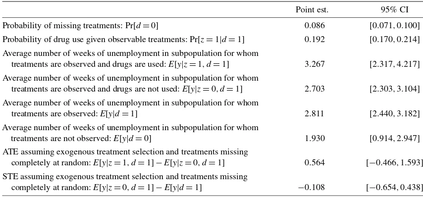
I focus attention on the 1345 (randomly sampled) respon-dents who were employed in 1983. Thus my empirical analy-sis concerns the subpopulation of persons who, in the nota-tion introduced in Secnota-tion2, have the shared observable covari-atex= {employed in 1983}(covariates left implicit in Secs.3 and4). Out of this group, 236 persons answered that they used drugs during work hours, 994 answered that they did not, and 115 refused to answer the question (8.55%). I take the out-come of interest to be the number of weeks that an individ-ual was unemployed during the calendar year 1983–1984. If the respondent answered the question on drug abuse (dj=1), then I observe whether she has been under the effect of drugs during work hours (zj=1|dj =1) or not (zj =0|dj =1); if the respondent skipped the question, the I register the missing data (dj=0). In the subpopulation of respondents, the average number of weeks of unemployment is relatively low regard-less of drug use. Abstracting from sample variability,E[y|z=
1,d =1] =3.267, and E[y|z=0,d =1] =2.703, whereas Pr[z=1|d=1] =0.192. If exogenous treatment selection (i.e.,
z⊥ {y(0),y(1)}) and ignorability of the observations with miss-ing treatment data (i.e.d⊥ {y(0),y(1),z}) is assumed, then it
Table 1. NLSY descriptive statistics (n=1345)
Point est. 95% CI
Probability of missing treatments: Pr[d=0] 0.086 [0.071,0.100]
Probability of drug use given observable treatments: Pr[z=1|d=1] 0.192 [0.170,0.214]
Average number of weeks of unemployment in subpopulation for whom
treatments are observed and drugs are used:E[y|z=1,d=1] 3.267 [2.317,4.217]
Average number of weeks of unemployment in subpopulation for whom
treatments are observed and drugs are not used:E[y|z=0,d=1] 2.703 [2.303,3.104]
Average number of weeks of unemployment in subpopulation for whom
treatments are observed:E[y|d=1] 2.811 [2.440,3.182]
Average number of weeks of unemployment in subpopulation for whom
treatments are not observed:E[y|d=0] 1.930 [0.914,2.947]
ATE assuming exogenous treatment selection and treatments missing
completely at random:E[y|z=1,d=1] −E[y|z=0,d=1] 0.564 [−0.466,1.593] STE assuming exogenous treatment selection and treatments missing
completely at random:E[y|z=0,d=1] −E[y|d=1] −0.108 [−0.654,0.438]
can be concluded that the ATE is equal to 0.564 weeks, and that the STE comparing a mandatory policy of no illegal drugs use to the status quo is equal to−0.108 weeks. This implies that not using drugs decreases the average number of weeks of unemployment in a calendar year by little more than one-half of a week compared with using drugs, and by a little more than one-tenth of a week compared with the status quo. Table1 summarizes these descriptive statistics, along with their 95% confidence intervals.
Testing for Missing Completely at Random and for Valid-ity of the Complete-Case Analysis. When facing missing-data problems as the one described earlier, researchers often con-duct “complete-case” analyses, in which observations with any missing values are simply discarded. In the context of treat-ment effects, when the treattreat-ment data are partially unobserv-able, this can lead to valid inference if (a) the treatment data are MCAR, (b)d⊥ {(y(0),y(1))|x}, and (c)d⊥ {(y(0),y(1),z)|x}.
Note that assuming thatP[y(t)|z,d,x] =P[y(t)|z,x]alone does
not imply validity of the CC analysis. Validity would be en-sured if it also is assumed that Pr(z=t|d,x)=Pr(z=t|x).
The assumptiond⊥ {(y(0),y(1))|x}, is not testable and
gener-ally does not seem appealing. For example, if Pr(z=t|d,x)=
Pr(z=t|x) and P[y(t)|z,d,x] =P[y(t)|z,x], then it follows
that P[y(t)|x,d =1] =P[y(t)|x,d=0]. Similarly, if Pr(z=
t|d,x)=Pr(z=t|x) and P[y(t)|z,d,x] =P[y(t)|z,x], then it
again follows thatP[y(t)|x,d=1] =P[y(t)|x,d=0].
On the other hand, a necessary condition for the assumption
d⊥ {(y(0),y(1),z)|x}and the MCAR assumption to hold can
be tested. In particular, the following result is easy to verify:
Lemma 7. Suppose thatd⊥ {(y(0),y(1),z)|x}. Then
P[y|d=1,x] =P[y|d=0,x]. (17)
Clearly, if the observability of the treatments is indepen-dent of the response functions and also of the received treat-ments conditional on the observed covariates, then, conditional on the observed covariates, the distribution of realized out-comes for the subpopulation for which the received treatments are observable should be the same as that for the subpopula-tion with missing treatment data. In practice, before conducting
CC analyses, one can test whether the equality in (17) holds. Note that if the assumptions P[y(t)|z,d,x] =P[y(t)|z,x] and
P(z|d,x)=P(z|x)are maintained, then condition (17) should
hold, and thus the same test as described in Lemma7 can be performed. But in both cases, condition (17) is necessary but not sufficient for the CC analysis to be valid or for the MCAR assumption to hold.
Given the NLSY sample, for x= {employed in 1983}, a Wilcoxon rank-sum test rejects the equality in (17) at the 5% significance level. Conditioning on additional covariates, the equality in (17) again can be rejected. For example, if we look at the group of respondents employed in 1983 who were younger than 23 and with at least a high school degree, then the null is rejected at 5% significance level.
6.2 Results
Tables2–4report respectively the bounds on the average out-come under a mandatory policy of no illicit drug use (MP(0)), the bounds on the ATE, and the bounds on the STE compar-ingMP(0)with the status quo, along with the Beresteanu and Molinari (2008; BM henceforth) 95% confidence intervals. The bounds are obtained under different sets of assumptions on (a) the ignorability of the missing treatments (complete cases vs all cases), (b) the probability of treatment for the subpopu-lation with missing treatments, and (c) treatment selection and treatment response. Before discussing the results, I briefly out-line how the confidence intervals are constructed.
Construction of the Confidence Intervals. Confidence inter-vals which asymptotically cover the identification regions de-rived in Sections3and4with a prespecified probability 1−α can be obtained using the results of BM (a conceptually differ-ent type of confidence regions that asymptotically cover the true parameter of interest, rather than its identification region, with probability at least 1−αcan be obtained by using the results of Imbens and Manski 2004). For the special case of interval identified parameters, as those studied in this article, Beresteanu and Molinari (2008, thm. 3.1) established the asymptotic equiv-alence between these confidence intervals, which are based on
Table 2. Bounds and BM CIs forE[y(0)]
Assumptions on treatment response and selection
No assumptions MTR MTR–MTS ETS
Complete cases [2.185, 12.162] [2.185, 2.811] [2.703, 2.811] 2.703 95% CI [1.2762, 13.0701] [1.8345, 3.1614] [2.3198, 3.1948] [2.3025, 3.1038]
All cases, with the following assumptions onp
p∈ [0,1] [1.998, 15.568] [1.998, 2.736] [2.472, 2.736] [2.473, 2.876] 95% CI [1.0478, 16.5180] [1.6647, 3.0691] [2.1155, 3.0927] [2.0996, 3.2500] p=1 [1.998, 15.568] [1.998, 2.736] [2.472, 2.736] 2.703
95% CI [1.0478, 16.5180] [1.6647, 3.0691] [2.1155, 3.0927] [2.3140, 3.0924] SAR [1.998, 15.568] [1.998, 2.736] [2.472, 2.736] [2.474, 2.876]
95% CI [1.0478, 16.5180] [1.6647, 3.0691] [2.1155, 3.0927] [2.1002, 3.2499] TMR [1.999, 12.140] [1.999, 2.736] [2.474, 2.736] [2.474, 2.676]
95% CI [1.0858, 13.0535] [1.6658, 3.0696] [2.1106, 3.0994] [2.1085, 3.0418] p=0 [2.163, 11.287] [2.163, 2.736] [2.637, 2.736] 2.623
95% CI [1.3196, 12.1303] [1.8290, 3.0699] [2.2780, 3.0952] [2.2612, 2.9850]
Table 3. Bounds and BM CIs for the ATE:E[y(1)] −E[y(0)]
Assumptions on treatment response and selection
No assumptions MTR MTR–MTS ETS
Complete cases [−11.535, 40.465] [0, 40.465] [0, 0.564] 0.564 95% CI [−12.6125, 41.5425] [0, 41.3918] [0, 1.4001] [−0.4659, 1.5933]
All cases, with the following assumptions onp
p∈ [0,1] [−14.995, 41.451] [0, 41.451] [0, 4.962] [−0.563, 1.389] 95% CI [−16.0626, 42.5191] [0, 42.2874] [0, 5.9571] [−1.4721, 2.2986]
p=1 [−14.830, 37.170] [0, 37.170] [0, 0.681] 0.126
95% CI [−15.9630, 38.3035] [0, 38.1396] [0, 1.4408] [−0.6850, 0.9367] SAR [−14.887, 40.760] [0, 40.760] [0, 1.366] [−0.563, 1.366]
95% CI [−15.9826, 41.8558] [0, 41.6815] [0, 2.2213] [−1.4802, 2.2837] TMR [−11.567, 40.760] [0, 40.760] [0, 1.366] [0.311, 1.366]
95% CI [−12.6443, 41.8378] [0, 41.6815] [0, 2.2267] [−0.6760, 2.3535]
p=0 [−10.714, 41.286] [0, 41.286] [0, 4.797] 0.644
95% CI [−11.7012, 42.2737] [0, 42.1271] [0, 5.7687] [−0.3617, 1.6494]
Table 4. Bounds and BM CIs for the STE:E[y(0)] −E[y]
Assumptions on treatment response and selection
No assumptions MTR MTR–MTS ETS
Complete cases [−0.628, 9.350] [−0.628, 0] [−0.108, 0] −0.108 95% CI [−1.4891, 10.2127] [−0.7808, 0] [−0.2696, 0] [−0.6540, 0.4376]
All cases, with the following assumptions onp
p∈ [0,1] [−0.738, 12.832] [−0.738, 0] [−0.264, 0] [−0.263, 0.140] 95% CI [−1.6890, 13.7826] [−0.8989, 0] [−0.4265, 0] [−0.4537, 0.3312] p=1 [−0.738, 12.832] [−0.738, 0] [−0.264, 0] −0.033
95% CI [−1.6890, 13.7826] [−0.8989, 0] [−0.4265, 0] [−0.2503, 0.1846] SAR [−0.738, 12.832] [−0.738, 0] [−0.264, 0] [−0.262, 0.140]
95% CI [−1.6890, 13.7826] [−0.8989, 0] [−0.4265, 0] [−0.4567, 0.3347] TMR [−0.737, 9.404] [−0.737, 0] [−0.262, 0] [−0.262,−0.060] 95% CI [−1.6044, 10.2716] [−0.9000, 0] [−0.4287, 0] [−0.4518, 0.1300] p=0 [−0.573, 8.551] [−0.573, 0] [−0.099, 0] −0.113
95% CI [−1.3897, 9.3674] [−0.7145, 0] [−0.2469, 0] [−0.2876, 0.0617]
inverting a Wald-type statistic, and the confidence intervals pro-posed by Chernozhukov, Hong, and Tamer (2007), which are based on inverting a QLR-type test statistic.
Denoting byϑˆLandϑˆUthe estimated lower and upper bound for a certain parameter of interest, withϑLandϑU their popu-lation counterparts, all what is required is that
√
dure. This confidence interval has the property that
lim
To use this result, one needs to establish the joint asymptotic normality of the sample analogs of each of the lower and up-per bounds obtained in Sections3and4. These results follow from standard arguments on the asymptotic properties of sam-ple means andL-statistics, and can be found in Molinari (2005, appendix B).
Discussion of the Results. Because the outcome of interest in this application is the number of weeks that an individual is unemployed in a calendar year, I setK0=0 andK1=52. In Tables 2–4, the first column of results corresponds to the case when nothing is assumed on the treatment response and selection mechanisms, the second column corresponds to the case when the MTR assumption is maintained, the third column corresponds to the case when the joint MTR–MTS assumption is maintained, and the fourth column corresponds to the case when the ETS assumption is maintained. As introduced in the previous section, these assumptions are specified as follows:
MTR : yj(1)≥yj(0), j∈J,
MTS : E[y(t)|z=1,d=i]
≥E[y(t)|z=0,d=i], t,i∈ {0,1}, ETS : E[y(t)] =E[y|z=t], t∈T.
In this application the MTR assumption states that each per-son’s unemployment outcome is weakly increasing in conjec-tured drug use during work hours.
The MTS assumption states that for allt∈ {0,1}, persons who do not select into using drugs during work hours have a weakly lower average number of weeks of unemployment compared with those who do select into using drugs during work hours. In other words, the MTS is a “sorting” assump-tion. In this application, it states that if we divide the popu-lation in two groups according to the received treatment, then the average outcome for the group that did not use drugs dur-ing work hours is lower than that for the group who did use drugs, for eacht∈T and for both the subpopulation with com-plete data and the subpopulation with missing treatment data. But because making use of it requires observations on the prob-ability of treatment, the MTS assumption can have identifying power onE[y(t)|d=0]only if prior information is available on Pr[z=1|d=0].
Manski and Pepper(2000) showed that the joint MTR–MTS assumption is a testable hypothesis that should be rejected if
E[y|z=u] is not weakly increasing inu. Table1 reports that in the NLSY sample,E[y|z=1,d=1] =3.267 and E[y|z=
0,d=1] = 2.703. The 95% confidence interval shows that the assumption that E[y|z=1,d =1] −E[y|z=0,d =1] ≥
0 cannot be rejected, and that the band contains everywhere monotone nondecreasing functions. Thus I proceed on the basis that the MTR–MTS assumption is consistent with the empirical evidence. The assumption cannot be tested for the subpopula-tion with missing treatment data, however.
The exogenous treatment selection assumption states that for allt∈ {0,1}, persons who select into treatmenttwould have ex-perienced the same average number of weeks of unemployment had they selected into treatment 1−t. Here this assumption is considered exclusively for illustrative purposes, because it is not very credible in this application.
The rows of Tables2–4correspond to different assumptions on the ignorability of the observations with missing treatments and on the probability of treatment. Comparing the bounds ob-tained under different combinations of assumptions allows us to disentangle the identification problems caused by the usual latent outcomes problem in the treatment effects literature and the additional problem of missing treatments.
Throughout this section, I focus mostly on the ATE, the ex-pected effect on unemployment of using illicit drugs during work hours for a person drawn randomly from the popula-tion. The ATE is the parameter of main interest in much of the empirical literature and often is estimated by ordinary least squares (OLS). Ignoring the observations with missing treat-ments, when empirical researchers suspect that there is positive selection into treatment (as it seems credible to assume in this application), they commonly take zero as a lower bound on the ATE and take the OLS estimate as an upper bound. Gonzalez-Luna(2005) showed that this informal practice corresponds to a model in which the MTR–MTS assumption is maintained. In particular, she showed that the bounds obtained under the MTR–MTS assumption are given by the interval from zero to the OLS estimate. Thus focusing on this parameter allows me to emphasize the extent to which this common practice may be misleading, in the presence of missing treatments. For compar-ison purposes, I also report the STE comparing the status quo with a mandatory policy of no illicit drug use.
Complete Cases. The first set of bounds and confidence in-tervals (CIs) is obtained assuming that the observations with missing treatment data can be ignored. With no assumptions on the treatment response and selection mechanism, the bounds are necessarily wide. This is due to the nonobservability of la-tent outcomes, which in this case implies that the bound on the ATE in Table 3 is of width(K1−K0)=52, whereas the bound on the STE in Table4and on theMP(0)in Table2 is equal to(K1−K0)Pr[z=1|d=1] =9.98. When the MTR and especially the joint MTR–MTS assumptions are imposed, the bounds shrink dramatically in width, as reported in the litera-ture. In particular, under the joint MTR–MTS assumption, ig-noring the observations with missing treatment data, one would conclude thatMP(0)would imply an average number of weeks of unemployment of 2.7–2.8 (2.3–3.2 if we look at the 95% CI). The ATE is 0–0.56 weeks (0–1.39 if we look at the 95% CI).
All Cases With p Unknown(p∈ [0,1]). The second set of bounds and CIs in each table is obtained when the observations with missing treatments are not ignored. To interpret the differ-ence in the results between the first and second sets in Tables 2–4, note that under the maintained assumption of ignorability of the observations with missing treatments, only the subsam-ple of observations with comsubsam-plete data is used (N=1230). In contrast, when nothing is assumed about the distribution of the missing treatments, all observations are used to draw inference (N=1345). But as long asp is unknown, no information can be extracted from the subsample with missing treatment data.
Because 80.8% of the respondents report that they have not been under the effect of drugs during work hours, the bounds on the average number of weeks of unemployment under MP(0) and the bounds on the STE are relatively narrow. Note that the bound is much wider if nothing is assumed about the distribu-tion of the missing treatments, in which case the width is 13.57 weeks, compared with if we assume ignorability of the obser-vations with missing treatment data, in which case the width is 9.98 weeks; that is, the width increases by 26% once we account for the missing treatments. Regarding the bound on the ATE, whereas when ignoring the observations with miss-ing treatment data, the width of the bound is equal to 52 weeks, when nothing is assumed about the distribution of missing treat-ments, the width increases to(1+Pr(d=0))K1=56.45.
Under the joint MTR–MTS assumption, considering the ob-servations with missing treatment data, one would conclude that
MP(0)implies an average number of weeks of unemployment of 2.47–2.74 (2.12–3.09 looking at the 95% CI). The STE indi-cates thatMP(0)implies a reduction in the average number of weeks of unemployment by up to 0.264 weeks. Observe that the upper bound on this effect is smaller than the upper bound ob-tained when ignoring the observations with missing treatment data. This result follows from the discussion in Section5.
Regarding the ATE, considering the missing treatments, we see that the effect ofMP(0)reduces average unemployment du-ration by up to 4.96 weeks (5.96 if we look at the 95% CI), com-pared with a mandatory policy of illicit drug use. Thus ignoring the observations with missing treatment data would imply up to an almost eightfold underestimation of this effect. Also note that when the selection problem is addressed through the MTR– MTS assumption, the missing-treatments problem becomes the main cause for the lack of identification. As with other missing-data problems, the additional degree of uncertainty caused by statistical considerations is relatively small compared with the identification problem.
All Cases With p=1. The third set of bounds and CIs in each table is obtained under the assumption that all respondents with missing treatment data have received the treatment, that is,p=1. In our example, this corresponds to the extreme as-sumption that all individuals who did not respond to the drug question did use drugs during work hours. This is a credible assumption if one believes in a very high level of stigma, in which all respondents engaging in an illicit activity refuse to answer survey questions about it, but none of the respondents not engaging in the illicit activity refuses to answer the ques-tions about it. This assumption does not have identifying power for the effect ofMP(0)or for the STE, because it implies that all outcomes are latent. But it does have strong identifying power
for the ATE, because it implies thatE[y(1)|d=0]is equal to
E[y|d=0] and thus is identified. When nothing is assumed on the treatment response and selection mechanism, the width of the bound shrinks back to be 52 weeks, although the en-tire sample is being considered. When the MTR assumption is maintained, the width of the bound decreases from 41.45 weeks when nothing is assumed onpto 37.17 weeks whenp=1; that is, the width decreases by 12%. When the joint MTR–MTS as-sumption is maintained, the width of the bound decreases from 4.96 weeks when nothing is assumed onpto 0.68 weeks when
p=1; that is, the width decreases by more than sevenfold.
All Cases With Stigma Affecting Response (i.e. p≥Pr[z=
1|d=1]). The fourth set of bounds and CIs in each table is obtained under the assumption that the probability that nonre-spondents used illicit drugs during work hours is at least as high as the probability that respondents did so, that is,p≥Pr[z=
1|d=1]. As discussed in Section3.3, when such a restriction is available, the bounds on the treatment effect of interest are ob-tained by taking the infimum and the supremum of the bounds derived in the previous section, overp∈ [Pr[z=1|d=1],1]. Similar to the previous case, this assumption does not have much identifying power for the effect of MP(0) or for the STE, because the infimum and the supremum of the bounds are achieved nearp=1. But it does have identifying power for the ATE. In particular, when the joint MTR–MTS assumption is maintained, the upper bound shrinks from 4.96 weeks when nothing is assumed onpto 1.37; that is, the width decreases by more than 3.5-fold.
All Cases With Treatments Missing at Random (i.e., p =
Pr[z=1|d=1]). The fifth set of bounds and CIs in each ta-ble is obtained under the TMR assumption. This assumption states that respondents who did not answer the question rela-tive to drug abuse are as likely as respondents who did answer the question to have been under the effect of drugs during work hours; it does not, however, imposed⊥(y(0),y(1),z). Given the NLSY sample, this assumption implies that Pr[z=1|d=
0] =0.192.
Under the TMR assumption, we get narrower bounds com-pared with the case of no assumptions onp, both on the aver-age number of weeks of unemployment underMP(0)and on the STE and ATE. In particular, for the ATE, we again con-clude that the decrease in the number of weeks of unemploy-ment stemming from a mandatory policy of no illicit drug use (compared to one of illicit drug use) is of up to 1.37 weeks (2.23 if we look at the 95% CI).
All Cases With p=0. The last set of bounds and CIs in each table is obtained under the assumption that all respondents with missing treatment data have not received the treatment, that is,
p=0. In our example this corresponds to the extreme assump-tion that all individuals who did not respond to the drug ques-tion did not use drugs during work hours. Here this assumpques-tion is considered exclusively for illustrative purposes, because it is not very credible in this empirical application. This assumption does have identifying power for the effect ofMP(0), because it implies thatE[y(0)|d=0]is equal toE[y|d=0]and thus is identified. When nothing is assumed on the treatment response and selection mechanism, the width of the bound shrinks to 9.12 weeks, as opposed to 13.57 when nothing is assumed on
p(a width reduction of 49%). When the joint MTR–MTS as-sumption is maintained, the width of the bound reduces from
![Table 3. Bounds and BM CIs for the ATE: E[y(1)] − E[y(0)]](https://thumb-ap.123doks.com/thumbv2/123dok/1134971.763201/10.594.64.519.308.493/table-bounds-bm-cis-ate-e-y-e.webp)
