07350015%2E2013%2E803866

(1)

Full Terms & Conditions of access and use can be found at

http://www.tandfonline.com/action/journalInformation?journalCode=ubes20

Download by: [Universitas Maritim Raja Ali Haji] Date: 11 January 2016, At: 22:12

Journal of Business & Economic Statistics

ISSN: 0735-0015 (Print) 1537-2707 (Online) Journal homepage: http://www.tandfonline.com/loi/ubes20

Realized Volatility Forecasting in the Presence of

Time-Varying Noise

Federico M. Bandi , Jeffrey R. Russell & Chen Yang

To cite this article: Federico M. Bandi , Jeffrey R. Russell & Chen Yang (2013) Realized Volatility

Forecasting in the Presence of Time-Varying Noise, Journal of Business & Economic Statistics, 31:3, 331-345, DOI: 10.1080/07350015.2013.803866

To link to this article: http://dx.doi.org/10.1080/07350015.2013.803866

Accepted author version posted online: 16 May 2013.

Submit your article to this journal

Article views: 305

(2)

Realized Volatility Forecasting in the Presence

of Time-Varying Noise

Federico M. BANDI

Johns Hopkins University, Baltimore, MD 21218, and Edhec-Risk, Nice 06202, France (fbandi1@jhu.edu)

Jeffrey R. RUSSELL

University of Chicago, Chicago, IL 60637 (jeffrey.russell@chicagobooth.edu)

Chen Y

ANG

Moody’s, New York, NY 10007 (michelle.chen.yang@gmail.com)

Observed high-frequency financial prices can be considered as having two components, a true price and a market microstructure noise perturbation. It is an empirical regularity, coherent with classical market microstructure theories of price determination, that the second moment of market microstructure noise is time-varying. We study the optimal, from a finite-sample forecast mean squared error (MSE) standpoint, frequency selection for realized variance in linear variance forecasting models with time-varying market microstructure noise. We show that the resulting sampling frequencies are generally considerably lower than those that would be optimally chosen when time-variation in the second moment of the noise is unaccounted for. These optimal, lower frequencies have the potential to translate into considerable out-of-sample MSE gains. When forecasting using high-frequency variance estimates, we recommend treating the relevant frequency as a parameter and evaluating itjointlywith the parameters of the forecasting model. The proposed joint solution is robust to the features of the true price formation mechanism and generally applicable to a variety of forecasting models and high-frequency variance estimators, including those for which the typical choice variable is a smoothing parameter, rather than a frequency.

KEY WORDS: Realized variance; Time-varying market microstructure noise; Volatility forecasting.

1. INTRODUCTION

The choice of sampling frequency, for realized variance, or bandwidth, for high-frequency kernel estimates of variance, should be dictated by finite-sample methods satisfying suit-able, statistical or economic, optimality criteria (Bandi and Russell 2006b). The existing finite-sample work has focused on the period-by-period (namedconditional,in this article) or unconditionalmean squared error (MSE) optimization of sam-pling frequency (Bandi and Russell2003,2008; Hansen and Lunde2006, and Oomen2006), for realized variance-type ob-jects, or smoothing parameter (Bandi and Russell2011), for high-frequency kernel estimates of variance. Joint considera-tion of the frequency/bandwidth selecconsidera-tion and forecasting prob-lem is important and was pursued by Andersen, Bollerslev, and Meddahi (2011), ABM hereafter, and Ghysels and Sinko (2011), GS henceforth. In the context of theoretical linear regression models with time-invariant noise, these contributions show that the optimal frequency selection problem, for the purpose ofR2

maximization or forecast MSE minimization, reduces, under as-sumptions, to the minimization of the unconditional variance of the realized variance estimator.

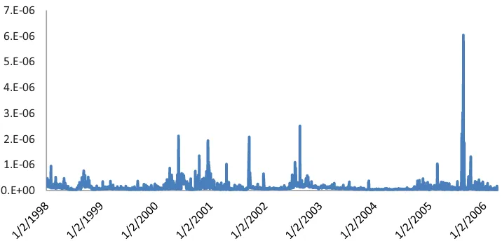
We re-examine the linear forecasting problem in ABM (2011) and GS (2011) under the assumption of time-variation in the second moment of market microstructure noise (for some early evidence, Bandi and Russell2006a; Oomen2006). This time-variation, illustrated graphically inFigure 1for our data, induces time-variation in the bias of the realized vari-ance estimator constructed using high-frequency data. A time-varying bias in realized variance should have implications for

forecasting when using realized variance as a predictor. Intu-itively, since the bias is not constant, it cannot be absorbed by the regression’s intercept. Hence, minimizing the variance of the regressor (i.e., realized variance), which is theR2_-maximizing

solution, under the assumption of a constant bias, may lead to ex-cessively high sampling frequencies and, in light of the one-to-one dependence between sampling frequency and bias contam-inations, large biases. Since these biases are time-varying, their dispersion may affect the quality of the forecasts. In essence, finite-sample optimality in the choice of sampling frequency, as given by theR2-maximizing solution if the noise is assumed to be time-varying, is likely to require a lower sampling frequency, so as to reduce time-changing bias contaminations, than previ-ously derived.

We make three contributions. First, in the context of a classi-cal price formation model with market microstructure noise to which we solely add noise time-variation (Section1), we for-malize the intuition mentioned earlier and deriveR2_-optimal

fre-quency selection methods for the joint frefre-quency selection and forecasting problem (Theorem 1). In this context, we find lower optimal frequencies than those derived when time-variation in the noise variance is unaccounted for. Interestingly, the new fre-quency choices are, in general, closer to those that would be obtained from the optimization of the finite-sample uncondi-tional MSE of the regressor (as in Bandi and Russell 2006a,

331

(3)

0.E+00 1.E-06 2.E-06 3.E-06 4.E-06 5.E-06 6.E-06 7.E-06

Time-varying noise second moment

Figure 1. Microstructure noise second moment’s estimates. We use Spiders midquotes on the NYSE. The sample period is 1998/1–2006/3. The online version of this figure is in color.

2008) than to those that would be obtained from the optimiza-tion of the uncondioptimiza-tional variance of the regressor as needed, for forecast MSE minimization, in linear forecasting models un-der the assumption of a constant noise second moment (ABM,

2011; GS,2011). In other words, we find that taking bias into account suboptimally (from the point of view of forecasting), through an unconditional MSE-based optimization, again under the assumption of a constant noise second moment, may be an empirically reasonable strategy.

Second, we emphasize that choosing the sampling fre-quency/bandwidth conditionally (for each entry/period in the regressor vector) rather thanunconditionally,as generally done in the literature, may be a superior strategy from a forecasting standpoint, even when the alternative is the exact, unconditional, R2_{-based optimal choice. Again, in the context of a classical}

price formation mechanism to which we only add noise time-variation, we find empirically verifiable conditions under which this statement is true.

Finally, we recognize that conditional choices may be em-pirically more cumbersome, in terms of implementation, than unconditional rules. In addition, the conditions under which they would outperform the optimal unconditional choice are, in general, model-specific and, when moving away from our illus-trative model to work with more complex specifications, hard to verify in practice. What we propose, instead, for empirical fore-casting work using high-frequency data is thejoint estimation of the optimal (from an R2 _{standpoint) frequency/bandwidth}

byleast-squares along with the parameters of the forecasting model. This solution coincides with the R2_-optimal,

closed-form, solution which we obtain in the context of our illustrative model, under the model’s assumptions, of course. However, the strategy (i) readily applies to any forecasting model mak-ing use of realized variance measures, (ii) is robust to features of the data such as noise dependence, dependence between the noise process and the true price1process, and dependence be-tween the true price variance and the noise variance; (iii) does

1_{The terminologies “true price” and “equilibrium price” are used}

interchange-ably in this article.

not require estimation of inputs, like the noise second moment variance or the quarticity, for empirical implementation; and (iv) can be broadly applied, by simply changing the choice vari-able from a frequency to a smoothing parameter, to all of the recently proposed kernel estimates of variance.

Several promising, recent contributions have studied vari-ance forecasting using microstructure noise-contaminated high-frequency variance estimates. These contributions have eval-uated the forecasting potential of the classical realized vari-ance estimator (Andersen et al. 2003; and Barndorff-Nielsen and Shephard2002) as well as that of classes of theoretically more robust, to noise, kernel-based estimators (e.g., Zhou1996; Zhang, Mykland, and A¨ıt-Sahalia 2005; Hansen and Lunde

2006; Barndorff-Nielsen et al.2008). Given time-series of alter-native variance estimates, the forecasts have generally been ob-tained using ARFIMA models (Bandi and Russell2008, 2011; Bandi, Russell, and Yang 2008), Mincer-Zarnowitz-style lin-ear regressions (ABM2004, 2011), or MIDAS-type regressions (GS 2006, 2011). Either statistical metrics, such as forecast MSEs and coefficients of determination (Corradi, Distaso, and Swanson2011; GS2006, 2010; A¨ıt-Sahalia and Mancini2008; ABM 2004, 2011) or economic metrics, such as the utility ob-tained by investors or the profits obob-tained by option traders on the basis of alternative variance forecasts (Bandi and Russell

2008,2011; Bandi, Russell, and Yang2008), have been used for the purpose of evaluating the quality of the forecasts. In all of these cases, necessary choice variables when working with high-frequency variance estimates are either the sampling high-frequency or the degree of smoothing implied by a bandwidth choice. In all cases, both the sampling frequency and the bandwidth can be selected, in agreement with the logic behind the least-squares solution to the linear forecasting problem presented in this arti-cle, to directly optimize the statistical or economic criterion of interest.

We work with a price formation mechanism, presented in Section1, which has been broadly adopted in the literature and is extended here solely to allow for a time-varying noise sec-ond moment. Similarly, we illustrate matters in the context of a simple, but commonly employed, autoregressive forecasting

(4)

model. Both choices are meant to derive closed-form, condi-tional and uncondicondi-tional, results and illustrate, through them, important conceptual issues pertaining to variance forecasting using realized variance measures when the noise variance is time-varying. The theoretical analysis will, however, lead us to our proposed, least-squares, unconditional solution to the choice problem which, as emphasized earlier and discussed in Section4, has general applicability and does not hinge either on the fine-grain features of the relation between noise and price process or on the forecasting model. In what follows, we use the symbol⊥⊥to signify “statistical independence.”

2. A CLASSICAL PRICE FORMATION MECHANISM AND FORECASTING MODEL

Consider a trading dayt. Assume availability ofM+1 eq-uispaced, observed logarithmic asset prices over [t, t+1] and write

pt+j δ = pt∗+j δ+ut+j δ j =0, . . . , M

or, in terms of continuously compounded returns,

pt+j δ−pt+(j−1)δ

wherep∗denotes theunobservabletrue price,udenotes unob-servablemarket microstructure noise, andδ=_M1 represents the time distance between adjacent price observations.

We assume the true price process evolves in time as a stochastic volatility local martingale, that is,p∗

t =

t 0σsdWs, where σt is a c`adl`ag stochastic volatility process, Wt is a standard Brownian motion, andσ ⊥⊥W (leverage effects are ruled out). The daily integrated variance is, therefore, defined asVt,t+1=

t+1

t σ

2

sds. From now on, we abuse notation a bit, when unambiguous, and sometime writeVtinstead ofVt,t+1for

brevity.

We assume the noise contaminations in the price processu are iid in discrete time, over each day, with mean zero, vari-ance σ_{t u}2, and fourth moment cuσ_{t u}4, where cu denotes kurto-sis. In addition,u⊥⊥p∗_and_σ2

t u⊥⊥Vt.2Importantly, the vari-ance of the market microstructure noise has a subscript t to signify that it can change from day to day. All other assump-tions are classical assumpassump-tions in this literature and, with the exception ofσ ⊥⊥W, which can be easily relaxed in asymp-totic designs, have been routinely employed when studying the finite sample and asymptotic properties of nonparametric esti-mates of integrated variance in the presence of noise (see, e.g., Bandi and Russell2003,2011; Barndorff-Nielsen et al.2008; Hansen and Lunde2006and Zhang, Mykland, and A¨ıt-Sahalia

2005, among others).3 While these conditions generally cap-ture important first-order effects in the data, the degree of their

2_{This assumption (}_σ2

t u⊥⊥Vt) can be easily relaxed. We will later show how the

optimal problem would change if the assumption were not satisfied.

3_{Bandi and Russell (}₂₀₀₃_,₂₀₀₈_{), A¨ıt-Sahalia et al. (2011), Oomen (}₂₀₀₅_,₂₀₀₆_),

and Hansen and Lunde (2006) discuss noise dependence. Kalnina and Linton (2008) allowed for a form of dependence between the noise and the true price.

empirical accuracy depends on the market structure, on the price measurement (transaction prices vs. midquotes, for example), as well as on the sampling scheme (calendar time vs. event time, for instance). Bandi and Russell (2006b) discussed these ideas.

As said, we depart from the “usual” assumptions by allowing for time-varying, across days, noise moments. This is the sense in which noise is time-varying. Sinceucaptures deviations of observed prices, midquotes, or transaction prices, from equilib-rium levels, time-variation in the noise moments is theoretically consistent, as is the case for bid/ask spread determination, with changing degrees of liquidity and asymmetric information (see, e.g., the discussion in Bandi and Russell 2005). Not only is the time-varying nature of the noise moments coherent with classical market microstructure theories of price formation, it is also—barring possible finite-sample contaminations in the corresponding estimates—a widely documented empirical reg-ularity (see Bandi and Russell2006aand Oomen2006, for some early evidence).

Assuming a constant second moment over a day, but allowing it to change from day to day, is a useful way to combine theoret-ical soundness with empirtheoret-ical tractability. As we discuss below, the time-varying second moments can be estimated consistently (nonparametrically) for each day in the sample. Alternatively, one could imagine a situation whereeachnoise contamination is endowed with a time-varying second moment.4 _{We leave}

the theoretical and empirical complications that this modeling choice would entail for future work.

We are interested in predicting Vt+1 given past daily

val-ues of the classical realized variance estimator, namely Vt =

M

j=1rt2+j δ (Barndorff-Nielsen and Shephard2002; Andersen et al. 2003). To this extent, it is useful to begin with a spe-cific model forming the basis for some of our analysis in the article. General results will be presented later. Assume Vt+1 =α+βVt+ξt+1, whereξt+1is such thatE(ξt+1|Ft)=0.

The model estimation is performed using lagged values ofVt, leading to the forecasting regression

Vt+1=α+βVt+ξt+1. (1)

The next section provides intuition about the main effects of time-varying noise on the sampling frequency and on the esti-mation of the model’s parameters.

2.1 Intuition

Under our assumed structure, the realized variance estimator takes the form

4_{In this case, the estimates may be readily interpreted as local daily averages.}

Importantly, the estimates can be further localized in the sense that, at the cost of decreased accuracy, the noise second moment can be estimated consistently, under the assumptions above, over any fixed intradaily period.

(5)

The estimator can also be rewritten as

We denote the estimation error with no market microstruc-ture noise by at=M_j₌₁r∗2

t+j δ−Vt. We define the difference between the realized bias on day t and the expected bias on daytas at =M_j₌₁ε2_t₊_{j δ}−Mσ_{t ε}2. The unconditional expected bias is given by ME(σ2

t ε) and the difference between the ex-pected day-tbias and the unconditional expected bias is given byM(σ2

t ε−E(σt ε2)). Finally, we denote the mean-zero, cross-product term byγt =2Mj=1rt∗+j δεt+j δ.

The forecast error of the estimated model in Equation (1) can now be expressed as

The sampling frequency only affects the second term in Equation (3) implying that the value ofM which minimizes the forecast error variance and the forecast MSE, or maximizes theR2, can be determined without consideration of the parameters of the forecasting model. Focusing on this second term, we note that the no noise case only yields var(at). This variance is minimized by choosing M as large as possible. The time-invariant noise case leads to var(at)+var(at)+var(γt), a convex function of the sampling frequency (Bandi and Russell 2003,2008). The solution to this minimization problem is the solution to the joint frequency and forecasting problem in the case of time-invariant noise (ABM,2011; GS,2011). The resulting optimal M is lower than the optimal M in the no noise case but, as we show formally in the next section, generally larger than the optimalMin the time-varying noise case due to the presence, in the latter case, of the extra termM2var(σ_{t ε}2). Equation (2), in fact, implies that a time-invariant noise second moment would have no impact on the regressor’s variance and would be absorbed by the regression’s intercept. It is, however, the variability in σ2

t ε which, when ignored, gives rise to larger-than-optimal M

choices and, through the quadratic termM2var(σ_{t ε}2), excessive dispersion of the regressor and the resulting forecast errors.

In sum,in all cases,the frequency which minimizes the fore-cast error variance coincides with the value which minimizes the variance of the regressor (Vt). The regressor’s variance for the time-varying noise case is, however, our focus.

The value ofβwhich minimizes the forecast error variance, instead, depends on the choice ofMand, hence, on the variance ofVt. Importantly, ifVt were observable, we would have

var(ξt+1)=(β−β)2var (Vt)+var(ξt+1)

and the theoretical solution to the problem would be classical:

and the theoretical least-squares βestimate is attenuated by theoptimized(overM) variance of the mean-zero measurement error component in realized variance, thereby givingβ < β .

Next, we consider theR2_{-optimal choice problem, for}_M_{, in}

the context of the simple model in this section. Specifically, we provide a discussion in terms of the model’sstructural param-eters. Near closed-form expressions will be used to facilitate interpretation before turning to a generally-applicable solution to the frequency choice and forecasting problem (in Section4).

2.2 Optimal Forecasting Frequencies: Closed-Form Expressions

Theorem 1 presents the optimal, unconditional, rule to choose the R2_{—maximizing number of observations} _M _{for the}

pro-posed, illustrative model with time-varying noise.

Theorem 1.Consider the regression in Equation (1). Under the assumptions made earlier on the data-generating process,

M1=arg maxRM2 =arg min

Remark 1.(Interpretation.) M1minimizes the unconditional

variance of the regressor (realized variance). Under an assump-tion of independence betweenσ_{t u}2 andVt,5this minimization translates into maximization of the forecasting regression’sR2

5_{If the assumption were not satisfied, then the solution would be:}

M

Given the proof of Theorem 1, the result is rather obvious.

(6)

(as in ABM2011; GS2011). The form of this unconditional variance is unusual and includes a term, of order M2_{, which}

accounts for the variability of the noise variance (i.e., the last term in Equation (5)).

Remark 2. (Implementation.) The quantitiesθt εandσ2 t ε can be estimated consistently, for each day in the sample, by us-ing sample moments of the observed return data sampled at the highest frequencies (Bandi and Russell2003, 2006a).6_Given

θt εandσ_{t ε}2, consistent estimates of the unconditional moments

E(θt ε),E(σ_{t ε}4),and var(σ_{t ε}2) can be obtained by employing sam-ple moments of the daily estimates under suitable stationarity assumptions. Estimation of the daily quarticityQt can be con-ducted by sampling the observed returns at relatively low (15-or 20-minute) frequencies.7_{Roughly unbiased estimates of the}

unconditional momentE(Qt) can then be derived by averag-ing the estimated daily quarticities under, again, an assumption of stationarity forQt. While empirical implementation of the method, by virtue of numerical minimization of the function in Equation (5), is fairly straightforward, the following Corollary provides a convenient, approximate rule to select the optimalM. When we compare it to similar rules in the literature, the new rule will help interpretation, to which we now turn.

Corollary to Theorem 1. For a large optimalM1,

M₁∗≈arg maxR_M2 =

Remark 3. The approximate rule in Equation (6) readily adapts to the noise variance’s variance. The larger this vari-ance relative to the signalE(Qt) generated by the underlying equilibrium price, the smaller the optimal number of observa-tions needed to computeV. As always in these problems, a smaller number of observations translates into smaller noise contaminations.

Remark 4. This rule differs from the optimal, in an uncondi-tional finite-sample MSE sense, approximate rule proposed by Bandi and Russell (2003,2008) in the presence of time-invariant noise, that is,

It also differs from the optimal (in anR2 sense), approximate rule proposed by ABM (2011) and GS (2011) in the case of time-invariant noise, that is,8

M₃∗=

6_{Bandi and Russell (}₂₀₀₇_{) discuss finite-sample bias corrections.}

7_{Bandi and Russell (}₂₀₀₈_{) discuss the empirical validity of this simple (albeit}

theoretically inefficient) procedure by simulation. Efficient estimation of the quarticity is an issue for future work. Important progress on this topic was recently made by Andersen, Dobrev, and Schaumburg (2010).

8_{Unsurprisingly, this is the same rule obtained by Bandi and Russell (}₂₀₀₃_{) in}

a different context, namely the finite-sample MSE (variance) minimization of their proposed bias-corrected realized variance estimator (Remark 8 in Bandi and Russell 2003 or Remark 4 in Bandi and Russell 2008).

The relative performance of these alternative rules depends on their relation withM∗

1. In general, M3∗> M2∗. This is easy to

1/2 _{under the above assumptions, but with}

a time-invariant noise second moment. Intuitively, because the noise-induced bias of the realized variance estimator increases drastically with the number of observations, the number of ob-servations which minimizes the unconditional MSE of realized variance is lower than the number of observations which mini-mizes its unconditional variance.

Importantly, if var(σ2

t ε)>(E(ε2))2 =(E(σt ε2))2 under time-varying noise, thenM∗

2 > M1∗. This last condition will be easily

satisfied for our data. Specifically, we will find thatM∗

3 > M2∗>

This result deserves attention. While a time-varying noise second moment can lead to relatively infrequent optimal sam-pling (M₁∗), optimizing the realized variance estimator’s uncon-ditional MSE, under the assumption of a constant noise variance, as implied byM₂∗, can be a superior strategy to focusing on the unconditional variance of realized variance, again under the as-sumption of a constant noise variance, as given by M∗

3. This

finding is particularly interesting since the latter choice would in fact be the optimal choice, from a forecast MSE standpoint, should the second moment of the noise, and the realized variance estimator’s bias, be assumed to be time-invariant.

While, in this section, we used rules-of-thumb to discuss the main issues, we emphasize that the empirical work, in Section

5, is conducted by optimizing the corresponding full-blown cri-teria. For example,M1 in Theorem 1 will be used in place of M∗

1 in the Corollary to Theorem 1.

3. CONDITIONALVERSUSUNCONDITIONAL FREQUENCY CHOICES

Rather than selecting one sampling frequency for all entries in the regressor vector (i.e., the vector of realized variance esti-mates), one could select a different (optimal) frequency for each entry/period. These period-by-period choices are named condi-tional.9 _{Bandi and Russell (}_2006a_,₂₀₀₈_{) used this approach,}

empirically, in predicting variance on the basis of autoregres-sive, fractionally integrated, models.

This section shows that the conditional approach has the po-tential to deliver superior forecasts than the unconditional ap-proach described in the previous section. In the context of our illustrative model, whether this is the case depends on empiri-cally verifiable conditions.

We consider the conditional finite-sample MSE-based ap-proximate rule in Bandi and Russell (2003,2008), that is,

M₂∗_t=

and compare it to the approximate optimal unconditional rule in Equation (6).

9_{In this literature, the term conditional is generally short for “conditional on the}

daily volatility path.”

(7)

Theorem 2. Define

Remark 5. The statement in Theorem 2 highlights the mo-ment condition affecting the preferability of an approximate conditional rule versus an approximate unconditional rule (see Equation (10)). Leaving aside issues related to estimation un-certainty, the inequality can be easily evaluated empirically by using the methods described in Remark 2 earlier.

Remark 6. Similarly, we can provide a statement for ex-actconditional and unconditional rules. Specifically, one could compare

where M1 is the exact R2—optimal number of observations

(from Theorem 1) and M2t is the exact, conditional, MSE-optimal number of observations from Bandi and Russell (2003,

2008). If Equation (12) is larger than Equation (11), then R_M22 _t > R_M12 . Naturally, this new inequality is slightly harder to verify than the inequality in the theorem. Its verification re-quires the solution ofT +1, whereTis the number of days in the sample, optimization problems to compute the relevantM’s (i.e.,M1andM2t witht=1, . . . , T). Analogous observations, and derivations, apply to the conditional, approximate minimum variance solution, namely

In both cases, the moment conditions yieldingR2_M 2t > R

M1are not satisfied for our data. Consistently, we will show that the in-sample MSEs delivered by conditional choices will, in general, be higher than those yielded by the optimal unconditional choices. However, the out-of-sample MSEs will, in some cases, be lower. We will return to these issues.

4. A GENERAL SOLUTION TO THE UNCONDITIONAL PROBLEM:JOINT LEAST-SQUARES OPTIMIZATION

Our previous discussion used a classical price formation mechanism, extended to allow for a time-varying noise sec-ond moment, as well as a traditional, albeit simple, forecasting model. Both choices were intended to obtain closed-form im-plications for important determinants of the optimal frequency choice when noise is time-varying. In this context, we have shown that there are sound theoretical reasons for choosing un-conditional sampling frequencies which are lower than those that would be optimally chosen in linear forecasting models when time-variation in the second moment of the noise is un-accounted for. We have also shown that suitable conditional choices have the potential to outperform theR2-optimal uncon-ditional solution.

While useful for understanding the main issues, the proposed unconditional rule hinges heavily on the assumed, illustrative model. Similarly, the conditions under which conditional choices are to be preferred are, in general, specific to the conditional rule being chosen (M2t or M3t, among other possible choices), the assumed data generating process, and the forecasting model. In all cases, the solutions we derived were intended to minimize the mean squared error of the residuals of the assumed forecasting regressions. We now show that this optimization may be conducted in full generality. Coherently with our previous logic, we now propose to address the optimal, unconditional, frequency/forecasting problemjointly with the model’s parameters.

To this extent, letVt+1=f(Vt, Vt−1, . . . , Vt−(K−1)|θ)+ξt+1

with E(ξt+1|Ft)=0 and define Vt+1=f(Vφ,t,Vφ,t−1, . . . ,

Vφ,t−(K−1)|θ)+ξt+1, for some function f(.|θ) and a specific

number of lagsK >0. We emphasize that the variance esti-mates Vφ,t are a function of φ. The parameter φ represents the number of observations (or a frequency), and is equal to M, in the case of realized variance. It denotes a bandwidth in

(8)

the case of high-frequency kernel estimates of variance, like Equation (14) later. The nonlinear least-squares solution to the joint forecasting/sampling problem is given by

(φ,θ)=arg min φ,θ

T

t=1

ξt+1

=arg min φ,θ

T

t=1

[Vt+1−f(Vφ,t,Vφ,t−1, . . . ,Vφ,t−(K−1)|θ)]2.

(13)

The approach has several appealing features. First, under the assumptions on the noise in Section2, iff(.) is consistent with an AR(1) model, the solution to the least-squares problem coin-cides with the theoretical solution in Theorem 1. More broadly, this solution is robust to potential noise dependence, depen-dence between the noise and the equilibrium price process, as well as dependence between the equilibrium price variance and the noise variance, as discussed in the previous section. Second, the forecasting model may be richer than an autoregression of any order. For instance, the joint approach readily applies to the MIDAS regressions in GS (2011), to the heterogeneous au-toregressive regressions (HAR) of Corsi (2009), possibly with leverage effects and jumps as in Corsi and Ren`o (2012), and to the HEAVY specifications in Shephard and Sheppard (2009),

among other approaches. In the next section, we apply it to an HAR specification. Third, the method does not require the evaluation of objects that are prone to finite-sample bias contam-inations, like the second moment of the noise and the quarticity. Finally, it encompasses all available high-frequency variance estimates, those for which the choice variable is a frequency and those for which the choice variable is a smoothing parame-ter. The issue of feasibility, which has to do with the empirical choice of regressand Vt+1, will be discussed in the following

applied section.

We note that the specification f(Vφ,t,Vφ,t−1, . . . ,

Vφ,t−(K−1)|θ) can be viewed as a mixed parameter model in

that φ is naturally defined over a discrete set. Under conven-tional assumptions (see, e.g., Ryu1999 and Choirat and Seri

2012), it is shown thatE(θi−θi0)2≤ζ T−1, for 0≤i≤G and

someζ >0, andE(φ−φ0)2≤ρT for some 0< ρ <1, where

the subscript 0 denotes (pseudo-)true values. In other words, the discrete parameter vectorφconverges (in mean square) to its theoretical counterpart at a faster, exponential, rate than the classical root T rate. In the context of our illustrative AR(1) model, the values θ=(θ2,θ1) are a slope and an intercept

estimate, respectively, consistent for the pseudo-true parame-tersβ0 in Equation (4) and α0 (see, Section2). As shown,β0

and α0 do not coincide with the parameters of the true

au-toregression. For instance, β0< β. In addition, φ is

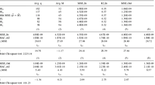
consis-Table 1. (AR, longer sample). We report forecasting regressions of integrated variance (estimated using optimally defined flat-top Bartlett kernels as in Bandi and Russell,2011) on one lag of realized variance. The regressor (realized variance) is sampled using the six methods described in the main text. We use Spiders midquotes on the NYSE. The sample period is 1/2002–3/2006. In all cases, 1000 observations are employed to estimate the model’s parameter and forecast. The table reports the choice of frequencyM, the average number of observations to be skipped for each sampling ruleq, in-sample and out-of-sample (one-step ahead) MSEs, and in-sampleR-squareds. It also reportst-statistics for the individual (in-sample and out-of-sample) MSEs,t-statistics for pairwise tests of equal (in-sample and out-of-sample) MSEs between choice (3) in the main text and all other choices, and a joint chi-squared test of equal (in-sample and out-of-sample) MSEs across sampling methods

Avg. q Avg. M MSE In R2 In MSE Out

M2t 162 32 4.66E-09 0.35 1.08E-09

M3t 117 45 4.52E-09 0.37 1.23E-09

Min MSE (φ=M) 118 45 4.55E-09 0.37 1.20E-09

M1 66 54 4.87E-09 0.32 1.39E-09

M2 62 56 4.86E-09 0.32 1.39E-09

M3 56 94 4.86E-09 0.32 1.38E-09

(1) (2) (3) (4) (5) (6)

MSE In 4.66E-09 4.52E-09 4.55E-09 4.87E-09 4.86E-09 4.86E-09

HAC std 1.66E-10 1.67E-10 1.63E-10 1.70E-10 1.69E-10 1.69E-10

t MSE 28.03 27.03 27.88 28.68 28.80 28.72

t13 t23 t43 t53 t63

t 18.76 −1.17 28.41 26.39 27.84

Joint Chi-square test: 2225.18

(1) (2) (3) (4) (5) (6)

MSE Out 1.08E-09 1.23E-09 1.20E-09 1.39E-09 1.39E-09 1.38E-09

HAC std 2.00E-10 3.01E-10 2.15E-10 2.23E-10 2.40E-10 2.11E-10

t MSE 5.40 4.10 5.59 6.22 5.79 6.57

t13 t23 t43 t53 t63

t −1.34 0.21 2.09 2.75 2.07

(9)

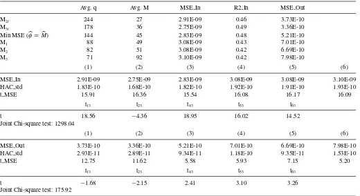
Table 2. (AR, shorter sample). We report forecasting regressions of integrated variance (estimated using optimally defined flat-top Bartlett kernels as in Bandi and Russell,2011) on one lag of realized variance. The regressor (realized variance) is sampled using the six methods described in the main text. We use Spiders midquotes on the NYSE. The sample period is 1/2004–3/2006. In all cases, 1000 observations are employed to estimate the model’s parameter and forecast. The table reports the choice of frequencyM, the average number of observations to be skipped for each sampling ruleq, in-sample and out-of-sample (one-step ahead) MSEs, and in-sampleR-squareds. It also reportst-statistics for the individual (in-sample and out-of-sample) MSEs,t-statistics for pairwise tests of equal (in-sample and out-of-sample) MSEs between choice (3) in the main text and all other choices, and a joint chi-squared test of equal (in-sample and out-of-sample) MSEs across sampling methods

M2t 244 27 2.91E-09 0.46 3.73E-10

M3t 178 36 2.75E-09 0.49 3.36E-10

Min MSE (φ=M) 144 45 2.83E-09 0.48 5.21E-10

M1 88 49 3.08E-09 0.43 7.01E-10

M2 82 51 3.08E-09 0.42 6.69E-10

M3 71 92 3.10E-09 0.42 7.98E-10

(1) (2) (3) (4) (5) (6)

MSE In 2.91E-09 2.75E-09 2.83E-09 3.08E-09 3.08E-09 3.10E-09

HAC std 1.83E-10 1.68E-10 1.82E-10 1.92E-10 1.91E-10 1.93E-10

t MSE 15.91 16.36 15.54 16.08 16.17 16.09

t13 t23 t43 t53 t63

t 18.56 −4.36 18.95 16.02 14.52

(1) (2) (3) (4) (5) (6)

MSE Out 3.73E-10 3.36E-10 5.21E-10 7.01E-10 6.69E-10 7.98E-10

HAC std 2.93E-11 2.89E-11 9.34E-11 1.18E-10 9.35E-11 1.53E-10

t MSE 12.75 11.62 5.58 5.93 7.15 5.20

t13 t23 t43 t53 t63

t −1.68 −2.15 2.41 3.10 3.26

tent for the value φ0 which minimizes, over the discrete set,

the variance of the estimated regressor, as shown in Theorem 1. The same logic applies to the general specificationf(Vφ,t,

Vφ,t−1, . . . ,Vφ,t−(K−1)|θ) for whichθ is a consistent estimate

of the attenuated pseudo-true parameter vectorθ0=θandφis

consistent, at the accelerated rateρ−1

2T, for the valueφ₀which minimizes the dispersion of the regressor matrix.

5. FORECASTING REGRESSIONS IN PRACTICE

This section examines the implications of theory with data. We use SPIDERS (Standard and Poor’s depository receipts) midquotes on the NYSE.10We remove quotes whose associated price changes and/or spreads are larger than 10%.

To render the regressions feasible (i.e., to evaluate the re-gressand Vt+1), we employ flat-top kernels as advocated by

10_{SPIDERS are shares in a trust which owns stocks in the same proportion as}

that found in the S&P 500 index. They trade like a stock (with the ticker symbol SPY on the Amex) at approximately one-tenth of the level of the S&P 500 index. They are widely used by institutions and traders as bets on the overall direction of the market or as a means of passive management. SPIDERS are exchange-traded funds. They can be redeemed for the underlying portfolio of assets. Equivalently, investors have the right to obtain newly issued SPIDERS shares from the fund company in exchange for a basket of securities reflecting the SPIDERS’ portfolio.

Barndorff-Nielsen et al. (2008). Write

V_tBNHLS =γ0+ q

s=1

ws(γs+γ−s), (14)

where γs =

M

j=1rt+j δrt+(j−s)δ with s= −q, . . . , q, ws = k(s−_q1), andk(.) is a function on [0,1] satisfyingk(0)=0 and k(1)=0. The well-known Bartlett kernel (k(x)=1−x), the cubic kernel (k(x)=1−3x2₊₂_x3_{), and the modified Tukey–}

Hanning kernel (k(x)=1−cosπ(1−x)2_/_{2), among other}

functions, satisfy the conditions onk(.).These estimators have favorable limiting properties under our price formation mech-anism (Barndorff-Nielsen et al. 2008).11 Furthermore, they have been shown to perform satisfactorily in practice (Bandi, Russell, and Yang2008and Bandi and Russell 2011). Impor-tantly, for each day in the sample, the estimators are unbiased under the assumptions in Section2. This is a useful property

11_If_q_∝_M2/3_,_{the estimators are consistent and converge to an asymptotic}

mixed normal distribution at speedM1/6. The additional requirementsk′₍₀₎₌₀

andk′(1)=0,combined withq∝M1/2, yield a faster rate of convergence (M1/4) to the estimators’ mixed normal distribution. The cubic kernel and the modified Tukey–Hanning kernel satisfy the extra requirements. See Barndorff-Nielsen et al. (2008) for further discussions.

(10)

Table 3. (HAR, longer sample). We report forecasting regressions of integrated variance (estimated using optimally defined flat-top Bartlett kernels as in Bandi and Russell,2011) on an HAR structure for realized variance. The regressor (realized variance) is sampled using the six

methods described in the main text. We use Spiders midquotes on the NYSE. The sample period is 1/2002–3/2006. In all cases, 1000 observations are employed to estimate the model’s parameter and forecast. The table reports the choice of frequencyM, the average number of

observations to be skipped for each sampling ruleq, in-sample and out-of-sample (one-step ahead) MSEs, and in-sampleR-squareds. It also reportst-statistics for the individual (in-sample and out-of-sample) MSEs,t-statistics for pairwise tests of equal (in-sample and out-of-sample)

MSEs between choice (3) in the main text and all other choices, and a joint chi-squared test of equal (in-sample and out-of-sample) MSEs across sampling methods

M2t 162 32 4.29E-09 0.41 9.77E-10

M3t 117 45 4.21E-09 0.42 9.85E-10

Min MSE (φ=M) 146 36 4.14E-09 0.43 1.11E-09

M1 66 54 4.33E-09 0.40 1.06E-09

M2 62 56 4.33E-09 0.40 1.05E-09

M3 56 94 4.33E-09 0.40 1.09E-09

(1) (2) (3) (4) (5) (6)

MSE In 4.29E-09 4.21E-09 4.14E-09 4.33E-09 4.33E-09 4.33E-09

HAC std 1.54E-10 1.53E-10 1.50E-10 1.54E-10 1.54E-10 1.54E-10

t MSE 27.82 27.54 27.53 28.10 28.19 28.20

t13 t23 t43 t53 t63

t 26.84 5.93 30.70 29.09 32.51

(1) (2) (3) (4) (5) (6)

MSE Out 9.77E-10 9.85E-10 1.11E-09 1.06E-09 1.05E-09 1.09E-09

HAC std 2.38E-10 2.36E-10 2.67E-10 2.27E-10 2.29E-10 2.20E-10

t MSE 4.10 4.18 4.15 4.66 4.56 4.96

t13 t23 t43 t53 t63

t −1.94 −0.87 −0.54 −0.73 −0.16

in that it guarantees, theoretically, at least, unbiasedness of the forecasts.12

In what follows, we use a Bartlett kernel and optimize the per-formance of the resulting estimates by using methods discussed in Bandi and Russell (2011). Specifically, for each day in the sample (i.e., conditionally, using our previous terminology), we select the number of autocovariancesq(or, equivalently, the smoothing sequence) to minimize the estimators’ finite-sample variance.13

We run regressions ofVBNHLS

t+1 on lagged realized variance. We

consider two forecasting models. The first model is consistent with our illustrative example and simply regressesVBNHLS

t+1 on

one past value of realized variance:

V_t,tBNHLS₊₁ =θ1+θ2VM,t−1,t +ξt+1.

12_{In general, of course, how to optimally trade off bias and variance of the}

forecasts depends on the adopted loss function. Since we are simply using kernel estimates to make the regressions feasible by empirically evaluating the regressand, it seems natural to employ unbiased estimators with favorable variance properties.

13_{Other estimators, such as the two-scale estimator of Zhang, Mykland, and}

A¨ıt-Sahalia (2005) and the multiscale estimator of Zhang (2006), also have favorable properties and could be used.

To capture more thoroughly the persistence properties of vari-ance, we also run HAR regressions as in Corsi (2009):

V_t,tBNHLS₊₁ =θ1+θ2VM,t −1,t +θ3VM,t −5,t +θ4VM,t −22,t+ξt+1,

whereVM,t −k,t =1_k

k

i=1VM,t −i,t−i+1fork≥1.

We consider two subsets of the data, the full period 1/2002– 3/2006 and the shorter 1/2004–3/2006 period.14In all cases, we use 1000 observations to estimate the model’s parameters and forecast (hence, our data starts in January 1998). We present in-sample and out-of-sample (one-step ahead) forecast MSEs along with related tests (zero MSE values and MSE equality between alternative regressors).

We report six choices ofM, leading to six different regressors. The first two are conditional, the remaining four are uncondi-tional. Even though rules-of-thumb are available for all optimal problems with the exception of our more general joint solu-tion in Equasolu-tion (3), the implementation is conducted, for the sake of superior accuracy, using the corresponding full-blown minimum problems. Coherently, as in the case ofM1versus its

14_{Results for the 1/2003–3/2006 period are qualitatively identical to those for}

the 1/2004–3/2006 period and are not provided for brevity.

(11)

approximate solutionM∗

1, we do not use asterisks to define the

Mchoices next.

1. M2tis theconditionalsolution to the minimum MSE problem in Theorem 2 of Bandi and Russell (2008)

2. M3t is the conditional solution to the minimum variance problem in Theorem 4 of Bandi and Russell (2008)

3. φ=M is the unconditional least-squares solution to the maximumR2problem or, equivalently, to the minimum fore-cast MSE problem in Equation (13)

4. M1 is the unconditionalsolution to the minimum variance

problem or, equivalently, the unconditional solution to the maximum R2 _{problem when the noise is time-varying in}

Theorem 1

5. M2is theunconditionalsolution to the minimum MSE

prob-lem under time-invariant noise, that is, the unconditional version of Theorem 2 in Bandi and Russell (2008)

6. M3 is the unconditionalsolution to the minimum variance

problem or, equivalently, the unconditional solution to the maximumR2 problem when the noise is time-invariant in ABM (2011) and GS (2011)

Tables1–4present results for the AR(1) model and the HAR model, respectively. We begin with the in-sample results. First,

we focus on theunconditional choices (3–6). For both fore-casting models and sample periods, we findφ=M < M 1< M2< M3. In other words, q3 < q2< q1<q, where q

indi-cates the average number of high-frequency observations to be skipped in the computation of the corresponding realized vari-ance estimator. Since, empirically, var(σ_{t ε}2)(=5.19e−14)> (E(σ_{t ε}2))2(=1.6e−14), the ranking of M values is consistent with the theoretical implications of the rules-of-thumb pre-sented in Section2. In essence, the variance of the noise sec-ond moment leads to variability in the forecast errors which can only be offset by a relatively small choice ofM, as is the case forφ=MandM1, so as to reduce the impact on the

ac-curacy of the forecasts of a time-changing realized variance’s bias.

By construction, the one-step choice 3 must, of course, yield a smaller in-sample MSE than those delivered by choices 4–6. Given a time-varying noise, one would not be surprised if this solution were not very dissimilar, in terms of corresponding MSE values, from the exact theoretical solutionM1in Equation

(4). In fact, under our illustrative model in Section2, the two choices would exactly coincide. For our data, the in-sample MSE values implied by Equations (4)–(6) are rather similar in spite of the variability of the corresponding sampling frequencies as implied by the alternativeMchoices. This outcome is evidence

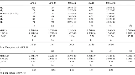
Table 4. (HAR, shorter sample). We report forecasting regressions of integrated variance (estimated using optimally defined flat-top Bartlett kernels as in Bandi and Russell,2011) on a HAR structure for realized variance. The regressor (realized variance) is sampled using the six

methods described in the main text. We use Spiders midquotes on the NYSE. The sample period is 1/2004–3/2006. In all cases, 1000 observations are employed to estimate the model’s parameter and forecast. The table reports the choice of frequencyM, the average number of

observations to be skipped for each sampling ruleq, in-sample and out-of-sample (one-step ahead) MSEs, and in-sampleR-squareds. It also reportst-statistics for the individual (in-sample and out-of-sample) MSEs,t-statistics for pairwise tests of equal (in-sample and out-of-sample)

MSEs between choice (3) in the main text and all other choices, and a joint chi-squared test of equal (in-sample and out-of-sample) MSEs across sampling methods

M2t 244 27 2.64E-09 0.51 2.05E-10

M3t 178 36 2.57E-09 0.52 2.22E-10

Min MSE (φ=M) 176 37 2.53E-09 0.54 2.30E-10

M1 88 49 2.68E-09 0.51 3.36E-10

M2 82 51 2.69E-09 0.50 3.12E-10

M3 71 92 2.69E-09 0.50 4.03E-10

(1) (2) (3) (4) (5) (6)

MSE In 2.64E-09 2.57E-09 2.53E-09 2.68E-09 2.69E-09 2.69E-09

HAC std 1.69E-10 1.62E-10 1.67E-10 1.70E-10 1.70E-10 1.71E-10

t MSE 15.60 15.92 15.14 15.71 15.76 15.77

t13 t23 t43 t53 t63

t 34.27 3.97 26.26 20.61 19.66

(1) (2) (3) (4) (5) (6)

MSE Out 2.05E-10 2.22E-10 2.30E-10 3.36E-10 3.12E-10 4.03E-10

HAC std 2.34E-11 2.54E-11 2.79E-11 7.66E-11 5.90E-11 9.98E-11

t MSE 8.74 8.74 8.25 4.39 5.30 4.04

t13 t23 t43 t53 t63

t −1.73 −0.55 1.56 1.67 1.93

(12)

Table 5. (Simulations, scenario (i)). We report forecasting regressions of integrated variance (estimated using optimally defined flat-top Bartlett kernels as in Bandi and Russell,2011) on one lag of realized variance. The regressor (realized variance) is sampled using the six methods described in the main text. We simulate second-by-second prices over 6.5 hr a day for 10 years using the model in the main text. One

thousand observations are employed to estimate the model’s parameter and forecast. The table reports the choice of frequencyM, the average number of observations to be skipped for each sampling ruleq, in-sample and out-of-sample (one-step ahead) MSEs, and in-sampleR-squareds.

It also reportst-statistics for the individual (in-sample and out-of-sample) MSEs,t-statistics for pairwise tests of equal (in-sample and out-of-sample) MSEs between choice (3) in the main text and all other choices, and a joint chi-squared test of equal (in-sample and

out-of-sample) MSEs

M2t 515 45 5.11E-09 0.82 1.29E-09

M3t 137 171 5.93E-09 0.82 1.05E-09

Min MSE (φ=M) 846 28 4.07E-09 0.85 1.37E-09

M1 639 37 6.38E-09 0.78 1.67E-09

M2 527 45 6.94E-09 0.76 1.85E-09

M3 272 86 1.01E-08 0.65 2.73E-09

(1) (2) (3) (4) (5) (6)

MSE In 5.11E-09 5.93E-09 4.07E-09 6.38E-09 6.94E-09 1.01E-08

HAC std 2.05E-10 2.55E-10 1.58E-10 2.58E-10 2.82E-10 4.09E-10

t MSE 24.92 23.21 25.71 24.71 24.63 24.62

t13 t23 t43 t53 t63

t 21.95 19.01 22.82 22.78 23.86

(1) (2) (3) (4) (5) (6)

MSE Out 1.29E-09 1.05E-09 1.37E-09 1.67E-09 1.85E-09 2.73E-09

HAC std 1.94E-10 1.54E-10 1.90E-10 2.45E-10 2.88E-10 3.56E-10

t MSE 6.66 6.82 7.21 6.84 6.42 7.67

t13 t23 t43 t53 t63

t −0.71 −3.04 2.20 2.45 6.66

of flatness in the in-sample MSE function across some, less than optimal, frequencies.

Turning toconditionalchoices, we find that using conditional MSE-optimal choices as in Equation (1) and, in some instances, conditional variance-optimal choices as in (2) does not perform in-sample as well as selecting only one frequency for all real-ized variance entries. As stressed earlier, the theoretical moment condition in Remark 6 is not satisfied for our data.

Statistically, for both forecasting models and sample periods, we find that (i) the in-sample MSEs are always different from zero, (ii) a chi-squared test of the null hypothesis of equal in-sample MSEs across sampling choices is easily rejected, and (iii) pairwiset-tests of the null of equal in-sample MSEs between the least-squares unconditional choice and other unconditional choices reject strongly and consistently.

We now turn to the out-of-sample (one-step ahead) results. First, for both forecasting models and sample periods again, the least-squares solution is generally preferable to the alternative unconditional solutions. This is especially true if the comparison is conducted with respect toM3, the minimum variance solution

under the assumption of a time-invariant noise, in Equation (6) (c.f.,t63). In the only instance in which the comparison is found

to be favorable toM3, that is, the HAR model over the longer

2002–2006 period, the statistical difference between the

result-ing out-of-sample MSEs is, however, determined to be very insignificant (t63= −0.16 inTable 3). Second, the conditional

solutions (1) and (2) are sometimes found to have favorable out-of-sample MSE properties. Both sets of findings, along with additional insights about the in-sample case, are discussed fur-ther by simulation in the next section.

6. MONTE CARLO ANALYSIS

We simulate the same equilibrium price process as in Huang and Tauchen (2005) and, more recently, Nolte and Voev (2012) but without jumps in the price process:

dp∗_t =exp(β0+β1vt)dW p∗

t p∗0 =0, dvt =αvvtdt+dW_tv v0=1/(−2αv),

whereWtp∗andWtvare, in agreement with the standard assump-tions in Section2, independent Brownian motions. As is typical in these problems, while empirically warranted, correlating the Brownian shocks does not affect our results in any meaningful way. The parameter vector is

β1=0.125, β0= β2

1

2αv, αv= −0.025.

(13)

Table 6. (Simulations, scenario (ii)). We report forecasting regressions of integrated variance (estimated using optimally defined flat-top Bartlett kernels as in Bandi and Russell,2011) on one lag of realized variance. The regressor (realized variance) is sampled using the six methods described in the main text. We simulate second-by-second prices over 6.5 hr a day for 10 years using the model in the main text. One

thousand observations are employed to estimate the model’s parameter and forecast. The table reports the choice of frequencyM, the average number of observations to be skipped for each sampling ruleq, in-sample and out-of-sample (one-step ahead) MSEs, and in-sampleR-squareds.

It also reportst-statistics for the individual (in-sample and out-of-sample) MSEs,t-statistics for pairwise tests of equal (in-sample and out-of-sample) MSEs between choice (3) in the main text and all other choices, and a joint chi-squared test of equal (in-sample and

out-of-sample) MSEs

M2t 815 29 2.74E-09 0.88 1.05E-09

M3t 258 91 4.17E-09 0.85 1.17E-09

Min MSE (φ=M) 815 29 3.80E-09 0.84 1.88E-09

M1 744 35 4.56E-09 0.80 2.22E-09

M2 603 43 4.75E-09 0.79 2.51E-09

M3 200 117 1.41E-08 0.51 9.41E-09

(1) (2) (3) (4) (5) (6)

MSE In 2.74E-09 4.17E-09 3.80E-09 4.56E-09 4.75E-09 1.41E-08

HAC std 9.79E-11 1.67E-10 1.38E-10 1.65E-10 1.70E-10 5.78E-10

t MSE 27.98 24.94 27.60 27.58 27.89 24.45

t13 t23 t43 t53 t63

t −26.55 12.18 23.44 26.47 23.45

(1) (2) (3) (4) (5) (6)

MSE Out 1.05E-09 1.17E-09 1.88E-09 2.22E-09 2.51E-09 9.41E-09

HAC std 1.35E-10 1.43E-10 1.62E-10 1.90E-10 1.83E-10 5.14E-10

t MSE 7.74 8.19 11.66 11.66 13.68 18.30

t13 t23 t43 t53 t63

t −9.34 −8.36 3.30 6.03 17.22

The noise processut is iidN(0, σ_{t u}2) within each day. The vari-ability of the noise second moment is generated in two ways. First, we define the noise second moment in terms of the multi-plication of empirically-reasonable, given our data and existing evidence, noise-to-signal ratios and the daily integrated variance of the true price process. Specifically,σ2

t u=θtVtwithθt=0.01 (high ratio) andθt =0.0001 (low ratio). Second, we do the same but replaceVtwith its expected valueE[Vt], which is equal to 1 under the model. In both cases, the high-ratio state (θt =0.01) is generated with likelihood 1/3. As emphasized, the noise second moment only changes from day to day and not from observation to observation within a day.

We sample the price process every second over 6.5 hr per day, 252 days per year, and over 10 years. The forecasting model is a simple autoregression. To summarize, we report two scenarios:15

15_{We provide here only a concise set of results. Among other things, we have}

(i) modified the model parameters (we have, for instance, allowed for correla-tion between the Brownian shocks), (ii) we have varied the noise variance by changing the probabilities as well as the size of the noise-to-signal ratios, (iii) we have sampled the process at lower 5-sec and 10-sec frequencies, and (iv) we have changed the forecasting model. In all cases, the findings were qualitatively unchanged. Results can be provided upon request.

(i) In the first scenario,σ_{t u}2 =θtVt. Since the dependence be-tweenσ_{t u}2 andVt is now apparent, we substituteM

1 for M1(as in footnote 5) as our frequency choice (4) to take

this dependence into account.16

(ii) In the second scenario, σ2

t u=θt. Our choice (4) contin-ues to be M1, that is, the unconditional solution to the

maximumR2_{problem when the noise is time-varying (as}

derived in Theorem 1).

Findings are presented in Table 5 (for scenario (i)) and

Table 6 (for scenario (ii)). As earlier, we begin with the in-sample results. In all cases, the least-squares optimal choice (3) leads to drastically lower sampling frequencies, and hence a smaller number of return observations, then the optimal choice under the assumption of a time-invariant noise in Equa-tion (6). The least-squares optimal choice is also generally closer to M1 or M1 than to M2 and M3. As with data, we

findM1(M1)< M2< M3and, in terms of the corresponding

16_{Importantly, the least-squares solution in Section}₄_{is immediately robust to}

this dependence.

(14)

in-sample MSE values, MSEM3 >MSEM2>MSEM1(MSEM1) with, of course, MSEM1(MSEM1)>MSEM. The ordering of the in-sample MSEs associated with unconditional choices is, as expected, more granular and clearer than with data.

As earlier with data, the conditional choices in Equations (1) and (2) have a tendency to yield larger in-sample MSE values than the optimal unconditional choice in Equation (3), but this is not always the case.

Statistically, we show, again, that (i) the in-sample MSEs are always different from zero, (ii) a chi-squared test of the null hypothesis of equal in-sample MSEs across different sam-pling choices is easily rejected, and (iii) pairwise t-tests of the null of equal in-sample MSEs between the least-squares un-conditional choice and other unun-conditional choices reject con-sistently. They do so more strongly when the alternative is choice (6).

Turning now to the out-of-sample outcomes, we find that the performance of the optimal least-squares choice is, as compared to the optimal unconditional choice under the assumption of a time-invariant noise, drastically superior both numerically and statistically (c.f.,t63=6.66 in scenario (i) andt63 =17.22 in

scenario (ii), where, as earlier, thetj h’s aret-statistics for pair-wise tests of equal MSEs across methodjand method h). As expected, the least-squares optimal MSE choice yields numer-ical results that are closer to those delivered by the remaining unconditional choices. Even in these cases, however, the numer-ical differences are in favor of the least-squares optimal MSE choice and are statistically significant. ComparingMtoM

1 and M1, for instance, we findt43 =2.2 in scenario (i) andt43 =3.3

in scenario (ii). As with data, the conditional choices in Equa-tions (1) and (2) outperform all unconditional choices, including the least-squares optimal choice.

7. CONCLUSIONS

Price formation mechanisms grounded in classical market microstructure theory imply that the second moment of market microstructure noise is time-varying. Empirical evidence read-ily confirms this implication of theory. We study the impact of noise time-variation on the forecasting of equilibrium price variance using realized variance. In the context of linear vari-ance forecasting models, we find the need for lower sampling frequencies than required when microstructure noise is assumed to be present but its variability is unaccounted for.

The goal of this article isnotto advocate a specific variance forecasting model. Choosing an optimal lag structure in the rel-evant forecasting regressions or enlarging the information set to allow for additional predictors are, among other extensions, im-portant issues beyond the scopes of the present article. Our goal is to use a well-understood price structure, as well as a classi-cal loss function amenable to the derivation of clear theoreticlassi-cal implications, to highlight conceptual aspects of the volatility forecasting problem in the presence of market microstructure noise which we regard as important. We show that account-ing for the time-varyaccount-ing nature of the noise moments through an unconditional least-squares solution which jointly selects the

frequency/bandwidth, along with the model’s parameters, is the-oreticallyR2_{-optimal and may be beneficial in practice from an}

out-of-sample standpoint. This solution is robust to the features of the true price formation mechanism and is generally applica-ble to any forecasting model and variance estimator, including those for which the relevant choice variable is a bandwidth, rather than a frequency.

While our focus has been on a well-understood statistical cri-terion, the same logic leading to a joint least-squares solution to the linear forecasting problem can be applied to suitable eco-nomic loss functions. The frequency/bandwidth choice problem can, in fact, be broadly cast in terms of the finite-sample opti-mization, along with the parameters of the forecasting model, of a variety of metrics of interest. This more general issue is better left for future work. and Theorem 4 in Bandi and Russell (2008), write

var(xt)=E(var(xt|σ, σu))+var(E(xt|σ, σu))

Proof of Theorem 2. Consider Equation (A.1). Plugging in the approximate optimal unconditional rule M∗

1 =( E(Qt)

var(σ2 t ε))

1/3_,

(15)

we obtain

. Using the MSE-optimal condi-tional rule in Bandi and Russell (2003,2008):

varM∗

We thank Torben Andersen, Nour Meddahi, two anonymous referees, the Co-Editor, Jonathan Wright, and seminar partic-ipants at the Imperial College Workshop on High-Frequency Data (London, February 22, 2007), the Conference on Volatility and High-Frequency Data (Chicago, April 21–22, 2007), and the 75th Cowles Foundation Anniversary Conference “Look-ing to the Future: A New Generation of Econometricians” (New Haven, June 11–12, 2007) for discussions. We are grateful to the

William S. Fishman Faculty Research Fund at Chicago Booth, University of Chicago, and Carey Business School, Johns Hop-kins University (Bandi), NYU Stern (Russell), and Chicago Booth, University of Chicago (Bandi, Russell, and Yang) for financial support.

[Received February 2011. Revised September 2012.]

REFERENCES

A¨ıt-Sahalia, Y., and Mancini, L. (2008), “Out-of-Sample Forecasts of Quadratic Variation,”Journal of Econometrics, 147, 17–33. [332]

A¨ıt-Sahalia, Y., Mykland, P., and Zhang, L. (2011), “Ultra High-Frequency Volatility Estimation With Dependent Microstructure Noise,”Journal of Econometrics, 160, 160–175. [333]

Andersen, T. G., Bollerslev, T., Diebold, F. X., and Labys, P. (2003), “Modeling and Forecasting Realized Volatility,”Econometrica, 71, 579–625. [332,333] Andersen, T. G., Bollerslev, T., and Meddahi, N. (2004), “Analytic Evaluation of Volatility Forecasts,”International Economic Review, 45, 1079–1110. [332]

——— (2011), “Realized Volatility Forecasting and Market Microstructure Noise,”Journal of Econometrics, 160, 220–234. [331,334,335,340] Andersen, T. G., Dobrev, D., and Schaumburg, E. (2010), “Integrated

Quar-ticity Estimation: Theory and Practical Implementation,” Working paper, Northwestern University, Federal Reserve Board of Governors and Federal Reserve Bank of New York. [335]

Bandi, F. M., and Russell, J. R. (2003), “Microstructure Noise, Realized Variance, and Optimal Sampling,” Working paper, University of Chicago. [331,333,334,335,336,344]

——— (2005), “Full-Information Transaction Costs,” Working paper, Univer-sity of Chicago. [333]

——— (2006a), “Separating Microstructure Noise From Volatility,”Journal of Financial Economics, 79, 655–692. [331,333,335]

——— (2006b), “Comment on Hansen and Lunde,”Journal of Business and Economic Statistics, 24, 167–173. [331,333]

——— (2007), “Volatility,” inHandbook of Financial Engineering, eds. J., Birge and V. Linetski, North Holland: Elsevier. [335]

——— (2008), “Microstructure Noise, Realized Variance, and Op-timal Sampling,” Review of Economic Studies, 75, 339–369. [331,332,333,334,335,336,340,343,344]

——— (2011), “Market Microstructure Noise, Integrated Variance Estimators, and the Accuracy of Asymptotic Approximations,”Journal of Econometrics, 160, 145–159. [331,332,333,338,339]

Bandi, F. M., Russell, J. R., and Yang, C. (2008), “Realized Volatility Forecasting and Option Pricing,”Journal of Econometrics, 147, 34–46. [332,338] Barndorff-Nielsen, O. E., Hansen, P., Lunde, A., and Shephard, N. (2008),

“Designing Realized Kernels to Measure Ex-Post Variation of Equity Prices in the Presence of Noise,”Econometrica, 76, 1481–1536. [332,333,338] Barndorff-Nielsen, O. E., and Shephard, N. (2002), “Econometric Analysis of

Realized Volatility and Its Use in Estimating Stochastic Volatility Models,” Journal of the Royal Statistical Society,Series B, 64, 253–280. [332,333] Choirat, C., and Seri, R. (2012), “Estimation in Discrete Parameter Models,”

Statistical Science, 27, 278–293. [337]

Corradi, V., Distaso, W., and Swanson, N. (2011), “Predictive Inference for Integrated Volatility,”Journal of the American Statistical Association, 106, 1496–1512. [332]

Corsi, F. (2009), “A Simple Approximate Long-Memory Model of Realized Volatility,”Journal of Financial Econometrics, 7, 174–196. [337,339] Corsi, F., and Ren`o, R. (2012), “Discrete-Time Volatility Forecasting With

Persistent Leverage Effect and the Link With Continuous-Time Volatility Modeling,”Journal of Business and Economic Statistics, 30, 368–380. [337] Ghysels, E., and Sinko, A. (2006), “Comment on Hansen and Lunde,”Journal

of Business and Economic Statistics, 24, 192–194. [332]

——— (2011), “Volatility Forecasting and Microstructure Noise,”Journal of Econometrics, 160, 257–271. [331,332,334,335,337,340]

Hansen, P. R., and Lunde, A. (2006), “Realized Variance and Market Microstruc-ture Noise” (with discussions),Journal of Business and Economic Statistics, 24, 127–161. [331,332,333]

Huang, X., and Tauchen, G. (2005), “The Relative Contribution of Jumps to Total Price Variance,” Journal of Financial Econometrics, 3, 456– 499. [341]

Kalnina, I., and Linton, O. (2008), “Estimating Quadratic Variation Consistently in the Presence of Correlated Measurement Error,”Journal of Econometrics, 147, 47–59. [333]

(16)

Nolte, I., and Voev, V. (2012), “Least-Squares Inference on Integrated Volatil-ity and the Relationship Between Efficient Prices and Noise,”Journal of Business and Economic Statistics, 30, 94–108. [341]

Oomen, R. C. A. (2005), “Properties of Bias-Corrected Realized Variance Under Alternative Sampling Schemes,”Journal of Financial Econometrics, 3, 555– 577. [331,333]

——— (2006), “Properties of Realized Variance Under Alternative Sampling Schemes,” Journal of Business and Economic Statistics, 24, 219–237. [331,333]

Ryu, K. (1999), “Econometric Analysis of Mixed Parameter Models,” Working Paper. [337]

Shephard, N., and Sheppard, K. (2009), “Realising the Future: Forecasting With High-Frequency Based (HEAVY) Volatility Models,”Journal of Applied Econometrics, 23, 197–231. [337]

Zhang, L. (2006), “Efficient Estimation of Stochastic Volatility Using Noisy Observations: A Multi-Scale Approach,”Bernoulli, 12, 1019–1043. [339]

Zhang, L., Mykland, P., and A¨ıt-Sahalia, Y. (2005), “A Tale of Two Time Scales: Determining Integrated Volatility With Noisy High-Frequency Data,” Jour-nal of the American Statistical Association, 100, 1394–1411. [332,333,339] Zhou, B. (1996), “High-Frequency Data and Volatility in Foreign-Exchange

Rates,”Journal of Business and Economic Statistics, 14, 45–52. [332]